Exponential families

Statistical Inference - PhD EcoStatData

Tommaso Rigon

Università degli Studi di Milano-Bicocca

Homepage

• This unit will cover the following topics:

  • One-parameter and multiparameter exponential families
  • Likelihood, inference, sufficiency and completeness
  • Exponential dispersion families

• The prime role of exponential families in the theory of statistical inference was first emphasized by Fisher (1934).

• Most well-known distributions—such as Gaussian, Poisson, Binomial, and Gamma—are instances of exponential families.

• Exponential families are the distributions typically considered when presenting the usual “regularity conditions”.

• With a few minor exceptions, this presentation will closely follow Chapters 5 and 6 of Pace and Salvan (1997).

Overview

• Figure 1 of Efron (2023). Three level of statistical modeling.

One-parameter exponential families

Exponential tilting

• Let Y be a non-degenerate random variable with support \mathcal{Y} \subseteq \mathbb{R} and density f_0(y) with respect to a dominating measure \nu(\mathrm{d}y).

• We aim at building a parametric family \mathcal{F} = \{f(;\theta) : \theta \in \Theta \subseteq \mathbb{R} \} with common support \mathcal{Y} such that f_0 is a special case, namely f_0 \in \mathcal{F}.

• A strategy for doing this is called exponential tilting, namely we could set f(y; \theta) \propto e^{\theta y}f_0(y). Thus, if f(y;\theta) is generated via exponential tilting, then f(y; 0) = e^0 f_0(y) = f_0(y).

• Let us define the mapping M_0:\mathbb{R}\rightarrow (0,\infty] M_0(\theta):=\int_\mathcal{Y}e^{\theta y}f_0(y)\nu(\mathrm{d}y), \qquad \theta \in \mathbb{R}. If M_0(\theta) is finite in a neighborhood of the origin, it is the moment generating function of Y.

• Moreover, we define the set \tilde{\Theta} \subseteq \mathbb{R} as the set of all \theta such that M_0(\theta) is finite, i.e. \tilde{\Theta} = \{\theta \in \mathbb{R} : M_0(\theta) < \infty\}.

Natural exponential family of order one

• The mapping K(\theta) = K_0(\theta) = \log{M_0(\theta)} is the cumulant generating function of f_0. It is finite if and only if M_0(\theta) is finite.

The parametric family generated via exponential tilting of f_0 \mathcal{F}_{\text{ne}}^1 = \left\{f(y;\theta) = \frac{e^{\theta y}f_0(y)}{M_0(\theta)} = f_0(y)\exp\{\theta y - K(\theta)\}, \quad y \in \mathcal{Y}, \theta \in \tilde{\Theta} \right\}, is called a natural exponential family of order one, and \tilde{\Theta} = \{\theta \in \mathbb{R} : K(\theta) < \infty\} is the natural parameter space.

• The natural parameter space \tilde{\Theta} is the widest possible and must be an interval; see exercises. The family \mathcal{F}_{\text{ne}}^1 is said to be full, whereas a subfamily of \mathcal{F}_{\text{ne}}^1 with \Theta \subseteq \tilde{\Theta} is non-full.

• By definition, all the densities f(y;\theta) \in \mathcal{F}_{\text{ne}}^1 have the same support.

A natural exponential family of order one, \mathcal{F}_{\text{ne}}^1, is said to be regular if \tilde{\Theta} is open.

Moment generating function

• In regular problems, the functions M_0(\theta) and K_0(\theta) associated to a r.v. Y with density f_0 are finite in a neighbor of the origin. A sufficient condition is that \tilde{\Theta} is an open set (regular \mathcal{F}_\text{en}^1).

Suppose M_0(t) < \infty for any |t| < t_0 and for some t_0 > 0. Then a standard result of probability theory (e.g. Billingsley (1995), Section 21) implies:

• The random variable Y has finite moments of all orders, i.e. \mu_k = \mathbb{E}(Y^k) < \infty for all k \geq 1.

• The moments (\mu_k)_{k \ge 1} and moment generating function M_0(t) uniquely characterize the law of Y and f_0. Moreover, M_0(t) admits a Taylor expansion around the origin: M_0(t) = 1 + \mu_1 t + \mu_2 \frac{t^2}{2!} + \mu_3 \frac{t^3}{3!} + \cdots = \sum_{k=0}^\infty \frac{t^k}{k!}\mu_k, \qquad |t| < t_0.

• The moments \mu_k equal the kth derivative of M_0(t) evaluated at the origin: \mu_k = \mathbb{E}_\theta(Y^k) = \frac{\partial^k}{\partial t^k} M_0(t) \Big|_{t = 0}, \qquad k \ge 1.

Cumulant generating function

Suppose K_0(t) = \log{M_0(t)} < \infty for any |t| < t_0 and for some t_0 > 0. Then:

• K_0 uniquely characterizes the law of Y and it admits a Taylor expansion K_0(t) = \kappa_1 t + \kappa_2 \frac{t^2}{2!} + \kappa_3 \frac{t^3}{3!} + \cdots = \sum_{k=1}^\infty \frac{t^k}{k!} \kappa_k, \qquad |t| < t_0, where the coefficients (\kappa_k)_{k \ge 1} are the cumulants of Y.

• The cumulants \kappa_k equal the kth derivative of K_0(t) evaluated at the origin \kappa_k = \frac{\partial^k}{\partial t^k} K_0(t) \Big|_{t = 0}, \qquad k \ge 1. Moreover, it can be shown the following moment relationships hold: \kappa_1 = \mathbb{E}_\theta(Y), \quad \kappa_2 = \text{var}_\theta(Y), \quad \kappa_3 = \mathbb{E}_\theta\{(Y - \mu_1)^3\}, \quad \kappa_4 = \mathbb{E}_\theta\{(Y - \mu_1)^4\} - 3\text{var}_\theta(Y)^2.

Refer to Pace and Salvan (1997), Section 3.2.5 for detailed derivations. Standardized cumulants \kappa_3/\kappa_2^{3/2} and \kappa_4/\kappa_2^2 are the skewness and the (excess of) kurtosis of Y.

Example: uniform distribution 📖

• Let Y \sim \text{Unif}(0,1) so that f_0(y) = 1 for y \in [0,1]. The exponential tilting of f_0 gives f(y; \theta) \propto e^{\theta y}f_0(y) = e^{\theta y}, \qquad y \in [0,1], \quad \theta \in \mathbb{R}.

• The normalizing constant, that is, the moment generating function, is M_0(\theta)= \mathbb{E}(e^{\theta Y}) = \int_0^1 e^{\theta y} \mathrm{d}y = \frac{e^\theta}{\theta}\Big|_0^1 = \frac{e^\theta - 1}{\theta}, \qquad \theta \neq 0. with M_0(0) = 1. Note that M_0 is continuous since \lim_{\theta \to 0}(e^\theta - 1)/\theta = 1.

• Consequently, we have M_0(\theta) < \infty for all \theta \in \mathbb{R} and the natural parameter space is \tilde{\Theta} = \mathbb{R}, which is an open set. The resulting density is f(y; \theta) = \frac{\theta e^{\theta y}}{e^{\theta -1}} = \exp\{\theta y - K(\theta)\}, \qquad y \in [0, 1], where K(\theta) = \log\{(e^\theta - 1)/\theta\}.

• It holds in general that \tilde{\Theta} = \mathbb{R} whenever f_0 has bounded support; thus, the family is regular.

Example: Poisson distribution 📖

• Let Y \sim \text{Poisson}(1) so that f_0(y) = e^{-1}/y! for y \in \mathbb{N}. The exponential tilting of f_0 gives f(y; \theta) \propto e^{\theta y}f_0(y) = \frac{e^{\theta y}e^{-1}}{y!}, \qquad y \in \mathbb{N}, \quad \theta \in \mathbb{R}.

• The normalizing constant, that is, the moment generating function, is M_0(\theta)= \mathbb{E}(e^{\theta Y}) = e^{-1}\sum_{k=0}^\infty \frac{e^{\theta y}}{y!} = \exp\{e^\theta - 1\}, \qquad \theta \in \mathbb{R}.

• Consequently, we have M_0(\theta) < \infty for all \theta \in \mathbb{R} and the natural parameter space is \tilde{\Theta} = \mathbb{R}, which is an open set. The resulting density is f(y; \theta) = \frac{e^{\theta y} e^{-1}}{y!}\frac{e^{-e^\theta}}{e^{-1}} = \frac{e^{-1}}{y!}\exp\{\theta y - (e^\theta - 1)\} = \frac{\lambda^y e^{\lambda}}{y!}, \qquad y \in \mathbb{N}, so that K(\theta) = e^\theta - 1 and having defined \lambda = e^\theta.

• In other words, the tilted density is again a Poisson distribution with mean e^\theta.

Example: exponential family generated by a Gaussian 📖

• Let Y \sim \text{N}(0,1) so that f_0(y) = 1/(\sqrt{2\pi})e^{-y^2/2} for y \in \mathbb{R}. The exponential tilting of f_0 gives f(y; \theta) \propto e^{\theta y}f_0(y) = \frac{1}{\sqrt{2\pi}}e^{\theta y -y^2/2}, \qquad y,\theta \in \mathbb{R}.

• The normalizing constant, that is, the moment generating function, is M_0(\theta)= \mathbb{E}(e^{\theta Y}) = \frac{1}{\sqrt{2\pi}}\int_\mathbb{R}e^{\theta y -y^2/2}\mathrm{d}y = e^{\theta^2/2}, \qquad \theta \in \mathbb{R}.

• Consequently, we have M_0(\theta) < \infty for all \theta \in \mathbb{R} and the natural parameter space is \tilde{\Theta} = \mathbb{R}, which is an open set. The resulting density is f(y; \theta) = \frac{1}{\sqrt{2\pi}}e^{\theta y}e^{-y^2/2}e^{-\theta^2/2} = \frac{e^{-y^2/2}}{\sqrt{2\pi}}\exp\{\theta y - \theta^2/2\} = \frac{1}{\sqrt{2\pi}}e^{-\frac{1}{2}(y - \theta)^2}, \qquad y \in \mathbb{R}, so that K(\theta) = \theta^2/2.

• In other words, the tilted density is again a Gaussian distribution with mean \theta.

Closure under exponential tilting 📖

• Let \mathcal{F}_{\text{ne}}^1 be an exponential family with parameter \psi and natural parameter space \tilde{\Psi}, with density f(y; \psi) = f_0(y)\exp\{\psi y - K(\psi)\}. The exponential tilting of f(y; \psi) gives f(y; \theta, \psi) \propto e^{\theta y} f(y; \psi) \propto f_0(y) \exp\{(\theta + \psi)y\}, and the normalizing constant of f_0(y) \exp\{(\theta + \psi)y\} is therefore
  \int_\mathcal{Y} f_0(y) \exp\{(\theta + \psi)y\} \, \nu(\mathrm{d}y) = M_0(\theta + \psi).

• Thus, for any \theta and \psi such that M_0(\theta + \psi) < \infty, the corresponding density is f(y; \theta, \psi) = f_0(y) \exp\{(\theta + \psi)y - K(\theta + \psi)\}, which is again a member of the exponential family \mathcal{F}_{\text{ne}}^1, with updated parameter \theta + \psi.

Exponential families are closed under exponential tilting, and \mathcal{F}_{\text{ne}}^1 can be thought of as being generated by any of its members.

Moments and cumulants

• The functions M_0(\theta) and K(\theta) = K_0(\theta) of a \mathcal{F}_\text{en}^1, refer to the baseline density f_0(y). Indeed, for any fixed \theta, the moment generating function of f(y; \theta) \in \mathcal{F}_\text{en}^1 is M_\theta(t) := \int_\mathcal{Y} e^{ty} f(y; \theta)\, \nu(\mathrm{d}y) = \frac{1}{M_0(\theta)} \int_\mathcal{Y} e^{(t + \theta)y} f_0(y)\, \nu(\mathrm{d}y) = \frac{M_0(t + \theta)}{M_0(\theta)}, \quad t + \theta \in \tilde{\Theta}.

• Consequently, the cumulant generating function of f(y; \theta) relates to K_0 as follows: K_\theta(t) = \log M_\theta(t) = K_0(t + \theta) - K_0(\theta), \quad t + \theta \in \tilde{\Theta}.

If \mathcal{F}_\text{en}^1 is a regular family, then \tilde{\Theta} is an open set, and \tilde{\Theta} = \text{int}\:\tilde{\Theta}, meaning that \theta is always an inner point of \tilde{\Theta}. Therefore, there exists a t_0 such that t + \theta \in \tilde{\Theta} for all |t| < t_0 implying that both M_\theta and K_\theta are well-defined.

If \mathcal{F}_\text{en}^1 is not regular, then for M_\theta(t) and K_\theta(t) to be well-defined, we require that \theta is not a boundary point; that is, \theta \in \text{int}\:\tilde{\Theta}, meaning it belongs to the interior of \tilde{\Theta}.

Textbooks sometimes suppress additive constants in defining K_0(\theta), e.g. using e^\theta instead of e^\theta-1. This is inconsequential (constants cancel in K_\theta(t)) but somewhat misleading.

Mean value mapping I

• Moments and cumulants exist for every \theta \in \text{int}\:\tilde{\Theta}. In particular, the cumulants are \kappa_k = \frac{\partial^k}{\partial t^k} K_\theta(t) \Big|_{t = 0} = \frac{\partial^k}{\partial t^k} \left[ K(t + \theta) - K(\theta) \right] \Big|_{t = 0} = \frac{\partial^k}{\partial \theta^k} K(\theta), \qquad k \ge 1.

Let Y \sim f(y; \theta), with f(y; \theta) \in \mathcal{F}_\text{en}^1. The first two moments of Y are obtained as: \mu(\theta) := \mathbb{E}_\theta(Y) = \frac{\partial}{\partial \theta} K(\theta), \qquad \text{var}_\theta(Y) = \frac{\partial}{\partial \theta} \mu(\theta) = \frac{\partial^2}{\partial \theta^2} K(\theta), We call \mu : \text{int}\:\tilde{\Theta} \to \mathbb{R} the mean value mapping.

• If f_0 is non-degenerate, then \text{var}_\theta(Y) > 0, implying that K(\theta) is a convex function, and \mu(\theta) is a smooth and monotone increasing, namely is a one-to-one map.

• Thus, if \mathcal{F}_\text{en}^1 is a regular exponential family, then \tilde{\Theta} = \text{int}\:\tilde{\Theta} and \mu(\theta) is a reparametrization.

Mean value mapping II

The mean value mapping has range \mathcal{M} = \text{Range}(\mu) = \{\mu(\theta) : \theta \in \text{int}\:\tilde{\Theta}\}. The set \mathcal{M} \subseteq\mathbb{R} is called mean space or expectation space.

Let C = C(\mathcal{Y}) be the closed convex hull of the sample space \mathcal{Y}, which is the smallest closed convex set C \subseteq \mathbb{R} containing \mathcal{Y}, namely: C(\mathcal{Y}) = \{ y \in \mathbb{R} : y = \lambda y_1 + (1 - \lambda)y_2, \quad 0 \le \lambda \le 1, \quad y_1,y_2 \in \mathcal{Y}\}.

• Hence, if \mathcal{Y} = \{0, 1, \dots, N\}, then C = [0,N]. If \mathcal{Y} = \mathbb{N}, then C = \mathbb{R}^+. If \mathcal{Y} = \mathbb{R}, then C = \mathbb{R}.

• Because of the properties of expectations, \mu(\theta) \in \text{int}\:C(\mathcal{Y}) for all \theta \in \text{int}\:\tilde{\Theta}, namely \mathcal{M} \subseteq \text{int}\:C(\mathcal{Y}). Indeed, \text{int}\:C(\mathcal{Y}) is an open interval whose extremes are the infimum and supremum of \mathcal{Y}.

Both definitions naturally generalize to the multivariate case when C, \mathcal{Y} \subseteq \mathbb{R}^p, for p > 1.

Mean value mapping III 📖

• In a regular exponential family, the mean value mapping \mu(\theta) is a reparametrization, meaning that for each \theta \in \tilde{\Theta}, there exists a unique mean \mu \in \mathcal{M} such that \mu = \mu(\theta).

• Moreover, in regular families, a much stronger result holds: for each value of y \in \text{int}\:C(\mathcal{Y}), there exists a unique \theta \in \tilde{\Theta} such that \mu(\theta) = y.

Theorem (Pace and Salvan (1997), Theorem 5.1)

If \mathcal{F}_\text{en}^1 is regular, then \Theta = \text{int}\:\tilde{\Theta} and \mathcal{M} = \text{int}\:C.

• This establishes a duality between the expectation space \mathcal{M} and the sample space. Any value in \text{int}\:C can be “reached”, that is, there exists a distribution f(y; \theta) with that mean.

• This correspondence is crucial in maximum likelihood estimation and inference.

This theorem can actually be strengthened: a necessary and sufficient condition for \mathcal{M} = \text{int}\:C is that the family \mathcal{F}_\text{en}^1 is steep (a regular family is also steep); see Pace and Salvan (1997).

A non regular and non steep exponential family

• Let us a consider an exponential family \mathcal{F}_\text{en}^1 generated by the density f_0(y) = c \frac{e^{-|y|}}{1 + y^4}, \qquad y \in \mathbb{R}. for some normalizing constant c > 0. The exponential tilting of f_0 gives f(y; \theta) \propto e^{\theta y}f_0(y) \propto \frac{e^{-|y| + \theta y}}{1 + y^4}, \qquad y \in \mathbb{R}, \quad \theta \in \tilde{\Theta}.
• The function M_0(\theta) is unavailable in closed form, however \tilde{\Theta} = [-1,1] since M_0(\theta) < \infty, \qquad \theta \in [-1, 1].
• Since \tilde{\Theta} is a closed set, the exponential family is not regular (and is not steep either). In fact, one can show that \lim_{\theta \to 1} \mu(\theta) = a < \infty, implying that \mathcal{M} = (-a, a), \qquad \text{ whereas } \qquad \text{int}\:C = \mathbb{R}.
• In other words, there are no values of \theta such that \mu(\theta) = y for any y > a, which implies, for instance, that the method of moments will encounter difficulties in estimating \theta.

Variance function I 📖

Let Y \sim f(y; \theta), with f(y; \theta) \in \mathcal{F}_\text{en}^1 and let \theta(\mu) be the inverse map of \mu(\theta). The variance of Y can be expressed as a function of \mu: V(\mu) := \text{var}_{\theta(\mu)}(Y) = \frac{\partial^2}{\partial \theta^2} K(\theta) \Big|_{\theta = \theta(\mu)}. The function V : \mathcal{M} \to \mathbb{R}^+ is called the variance function of the exponential family \mathcal{F}_\text{en}^1.

• The importance of the variance function V(\mu) is related to the following characterization result due to Morris (1982).

Theorem (Pace and Salvan (1997), Theorem 5.2)

If Y has a density that belongs to a \mathcal{F}_\text{en}^1, then the pair (\mathcal{M}, V(\mu)) uniquely determine the natural parameter space \tilde{\Theta} and the cumulant generating function K(\theta), and hence also f(y;\theta).

Variance function II 📖

• The characterization theorem of Morris (1982) is constructive in nature, as its proof provides a practical way of determining K(\theta) from (\mathcal{M}, V(\mu)). In particular, the function K(\cdot) must satisfy K\left(\int_{\mu_0}^\mu \frac{1}{V(m)}\mathrm{d}m\right) = \int_{\mu_0}^\mu \frac{m}{V(m)}\mathrm{d}m, where \mu_0 is an arbitrary point in \mathcal{M}.

• For example, let \mathcal{M} = (0, \infty) and V(\mu) = \mu^2. Then, choosing \mu_0=1 gives K\left(1 - \frac{1}{\mu}\right) = \log\mu, and therefore \theta(\mu) = 1 - 1/\mu, giving \tilde{\Theta} = (-\infty, 1) and \mu(\theta) = (1 - \theta)^{-1}. Hence we obtain K(\theta) = -\log(1 - \theta), which corresponds to the exponential density f_0(y) = e^{-y}, for y > 0.

In order to identify \mathcal{F}_\text{en}^1 both \mathcal{M} and V(\mu) must be known.

Well-known exponential families

Notation	\text{N}(\psi, 1)	\text{Poisson}(\psi)	\text{Bin}(N, \psi)	\text{Gamma}(\nu,\psi), \nu > 0
\mathcal{Y}	\mathbb{R}	\mathbb{N}	\{0, 1, \dots, N\}	(0, \infty)
Natural param.
\theta(\psi)	\psi	\log{\psi}	\log\{\psi/(1 - \psi)\}	-\psi
f_0(y)	(\sqrt{2\pi})^{-1}e^{-\frac{1}{2}y^2}	e^{-1}/ y!	\binom{N}{y}\left(\frac{1}{2}\right)^N	y^{\nu - 1}e^{-y}/\Gamma(\nu)
K(\theta)	\theta^2/2	e^\theta-1	N \log(1 + e^\theta) - N\log{2}	-\nu \log(1-\theta)
\tilde{\Theta}	\mathbb{R}	\mathbb{R}	\mathbb{R}	(-\infty, 0)
Mean param.
\mu(\theta)	\theta	e^\theta	N e^\theta/(1 + e^{\theta})	-\nu/\theta
\mathcal{M}	\mathbb{R}	(0, \infty)	(0, N)	(0, \infty)
V(\mu)	1	\mu	\mu(1 - \mu/ N)	\mu^2/\nu

Quadratic variance functions

• There is more in Morris (1982)’s paper. Specifically, he focused on a subclass of quadratic variance functions, which can be written as V(\mu) = a + b\mu + c\mu^2, for some known constants a, b, and c.

• Morris (1982) showed that, up to transformations such as convolution, there exist only six families within \mathcal{F}_\text{en}^1 that possess a quadratic variance function. These are: (i) the normal, (ii) the Poisson, (iii) the gamma, (iv) the binomial, (v) the negative binomial, and (vi) a sixth family.

• The sixth (less known) distribution is called the generalized hyperbolic secant, and it has density f(y; \theta) = \frac{\exp\left\{\theta y - \log\cos{\theta}\right\}}{2\cosh(\pi y/2)}, \qquad y \in \mathbb{R}, \quad \theta \in (-\pi/2, \pi/2), with mean function \mu(\theta) = \tan{\theta} and variance function V(\mu) = \csc^2(\theta) = 1 + \mu^2, and \mathcal{M} = \mathbb{R}. It is also a regular exponential family.

A general definition of exponential families I

Let h(y) > 0, s(y), be real-valued functions not depending on \psi and let \theta(\psi), G(\psi) be real-valued functions not depending on y. The parametric family \mathcal{F}_{\text{e}}^1 = \left\{f(y;\psi) = h(y)\exp\{\theta(\psi) s(y) - G(\psi)\}, \quad y \in \mathcal{Y}\subseteq \mathbb{R}, \: \psi \in \Psi \right\}, is called a exponential family of order one, where the normalizing constant is \exp{G(\psi)} = \int_\mathcal{Y} h(y) \exp\{\theta(\psi) s(y)\} \nu(\mathrm{d}y). The family is full if the parameter space \Psi is the widest possible \tilde{\Psi} = \{\psi \subseteq\mathbb{R}: G(\psi) < \infty\}.

Suppose f(y; \psi) \in \mathcal{F}_\text{e}^1. Then, the function \theta(\psi) must be a one-to-one mapping, that is, a reparametrization, otherwise, the model would not be identifiable. Hence, we can write: f(y; \psi) = h(y)\exp\{\theta(\psi) s(y) - \tilde{G}(\theta(\psi))\}, for some function \tilde{G}(\cdot) such that G(\psi) = \tilde{G}(\theta(\psi)).

A general definition of exponential families II

• When s(y) is an arbitrary function of y, then \mathcal{F}_\text{e}^1 is broader than \mathcal{F}_\text{en}^1.

• Without loss of generality, we can focus on the natural parametrization \theta \in \Theta and a density baseline h(y) = f_0(y), meaning that f(y;\theta) \in \mathcal{F}_\text{e}^1 can be written as f(y; \theta) = f_0(y)\exp\{\theta s(y) - K(\theta)\}, because the general case would be a reparametrization of this one.

• Let Y \sim f(y; \theta), with f(y; \theta) \in \mathcal{F}_\text{e}^1. Then, the random variable S = s(Y) has density f_S(s; \psi) = \tilde{f}_0(s)\exp\{\theta s - K(\theta)\}, for some baseline density \tilde{f}_0(s), namely f_S(s; \psi) \in \mathcal{F}_\text{en}^1. If in addition s(y) is a one-to-one invertible mapping, this means Y = s^{-1}(S) is just a transformation of an \mathcal{F}_\text{en}^1.

A full exponential family \mathcal{F}_\text{e}^1 is, technically, a broader definition, but in practice it leads to a reparametrization of a natural exponential family \mathcal{F}_\text{en}^1 in a transformed space s(Y).

Multiparameter exponential families

Natural exponential families of order p

• Let Y be a non-degenerate random variable with support \mathcal{Y} \subseteq \mathbb{R}^p and density f_0(y) with respect to a dominating measure \nu(\mathrm{d}y).

• Let us define the mapping M_0:\mathbb{R}^p\rightarrow (0,\infty] M_0(\theta):=\int_\mathcal{Y}e^{\theta^T y}f_0(y)\nu(\mathrm{d}y), \qquad \theta \in \mathbb{R}^p.

The parametric family generated via exponential tilting of a density f_0 \mathcal{F}_{\text{ne}}^p = \left\{f(y;\theta) = \frac{e^{\theta^T y}f_0(y)}{M_0(\theta)} = f_0(y)\exp\{\theta^T y - K(\theta)\}, \quad y \in \mathcal{Y}\subseteq \mathbb{R}^p, \:\theta \in \tilde{\Theta} \right\}, is called a natural exponential family of order one, K(\theta) = \log M_0(\theta) and \tilde{\Theta} = \{\theta \in \mathbb{R}^p : K(\theta) < \infty\} is the natural parameter space.

• The family \mathcal{F}_{\text{ne}}^p is said to be full, whereas a subfamily of \mathcal{F}_{\text{ne}}^p with \Theta \subseteq \tilde{\Theta} is non-full. Moreover, the family \mathcal{F}_{\text{ne}}^p is said to be regular if \tilde{\Theta} is an open set.

Example: multinomial distribution I 📖

• Let Y = (Y_1,\dots,Y_{p-1}) \sim \text{Multinom}(N; 1/p,\dots,1/p) be a multinomial random vector with uniform probabilities, so that its density f_0 is
  f_0(y) = \frac{N!}{y_1!\cdots y_p!}\left(\frac{1}{p}\right)^N, \qquad y = (y_1,\dots,y_{p-1}) \in \mathcal{Y} \subseteq \mathbb{R}^{p-1}, where \mathcal{Y} = \{(y_1,\dots,y_{p-1}) \in \{0,\dots,N\}^{p-1} : \sum_{j=1}^{p-1} y_j \le N\}, having set y_p := N - \sum_{j=1}^{p-1} y_j.

• The exponential tilting of f_0 yields f(y; \theta) \propto f_0(y) e^{\theta^T y} = \frac{N!}{y_1!\cdots y_p!}\left(\frac{1}{p}\right)^N e^{\theta_1 y_1 + \cdots + \theta_{p-1} y_{p-1}}, \qquad y \in \mathcal{Y}, \;\theta \in \mathbb{R}^{p-1}.

• As a consequence of the multinomial theorem, the normalizing constant, that is, the moment generating function, is
  M_0(\theta) = \mathbb{E}\left(e^{\theta^T Y}\right) = \left(\frac{1}{p}\right)^N(1 + e^{\theta_1} + \cdots + e^{\theta_{p-1}})^N. Thus M_0(\theta) < \infty for all \theta \in \mathbb{R}^{p-1} and the natural parameter space is the open set \tilde{\Theta} = \mathbb{R}^{p-1}.

Example: multinomial distribution II 📖

• The resulting tilted density is f(y; \theta) = f_0(y)e^{\theta^Ty - K(\theta)} = \frac{N!}{y_1!\cdots y_p!}\frac{e^{\theta_1 y_1 + \cdots + \theta_{p-1}y_{p-1}}}{(1 + e^{\theta_1} + \cdots + e^{\theta_{p-1}})^N}, where K(\theta) = \log{M_0(\theta)} = N\log(1 + e^{\theta_1} + \cdots + e^{\theta_{p-1}}) - N\log{p}.

• In other words, the tilted density is again a multinomial distribution with parameters N and probabilities \pi_j = e^{\theta_j} / (1 + e^{\theta_1} + \cdots + e^{\theta_{p-1}}). In fact, we can write: \begin{aligned} f(y; \theta) &= \frac{N!}{y_1!\cdots y_p!}\frac{e^{\theta_1 y_1} \cdots e^{\theta_p y_p}}{(\sum_{j=1}^p e^{\theta_j})^{y_1} \cdots (\sum_{j=1}^p e^{\theta_j})^{y_p}} = \frac{N!}{y_1!\cdots y_p!} \prod_{j=1}^p\left(\frac{e^{\theta_j}}{\sum_{k=1}^p e^{\theta_k}}\right)^{y_j} \\ &= \frac{N!}{y_1!\cdots y_p!} \prod_{j=1}^p\pi_j^{y_j}. \end{aligned} where we defined \theta_p := 0, so that \sum_{j=1}^pe^{\theta_j} = 1 + e^{\theta_1} + \cdots + e^{\theta_{p-1}}, recalling that \sum_{j=1}^py_j = N.

• The tilted density belongs to a regular natural exponential family \mathcal{F}_\text{en}^{p-1} of order p-1.

Example: independent exponential families 📖

• Let Y = (Y_1,\dots,Y_p) be a random vector of independent random variables each belonging to a full natural exponential family \mathcal{F}_\text{en}^1 of order 1, with density f(y_j; \theta_j) = f_j(y_j)\exp\{\theta_j y_j - K_j(\theta_j)\}, \qquad \theta_j \in \tilde{\Theta}_j.

• Let \theta = (\theta_1,\dots,\theta_p). Because of independence, the joint distribution of Y is \begin{aligned} f(y;\theta) &= \prod_{j=1}^p f(y_j;\theta_j) = \prod_{j=1}^pf_j(y_j)\exp\{\theta_j y_j - K_j(\theta_j)\} \\ &= \left[\prod_{j=1}^pf_j(y_j)\right]\exp\left\{\sum_{j=1}^p\theta_jy_j - \sum_{j=1}^pK_j(\theta_j)\right\} \\ & = f_0(y)\exp\{\theta^Ty - K(\theta)\} \end{aligned} where f_0(y) = \prod_{j=1}^pf_j(y_j), K(\theta) = \sum_{j=1}^pK_j(\theta_j) and the natural parameter space is \tilde{\Theta} = \tilde{\Theta}_1 \times \cdots \times \tilde{\Theta}_p.

• Thus, f(y;\theta) is an \mathcal{F}_\text{en}^p, in which K(\theta) is a separable function.

Mean value mapping and other properties

• Let Y \sim f(y; \theta), with f(y; \theta) \in \mathcal{F}_\text{en}^p. The cumulant generating function is
  K_\theta(t) = \log M_\theta(t) = K_0(t + \theta) - K_0(\theta), \qquad t + \theta \in \tilde{\Theta}. In particular, the first two moments of Y are obtained as:
  \mu(\theta) := \mathbb{E}_\theta(Y) = \frac{\partial}{\partial \theta} K(\theta), \qquad \text{var}_\theta(Y) = \frac{\partial}{\partial \theta^\top} \mu(\theta) = \frac{\partial^2}{\partial \theta \partial \theta^\top} K(\theta),

• If f_0 is non-degenerate, then the covariance matrix \text{var}_\theta(Y) is positive definite, implying that K(\theta) is a convex function, and \mu(\theta) is a smooth one-to-one map.

• The definitions of mean value mapping \mu(\theta), its range \mathcal{M}, the convex hull C(\mathcal{Y}) of the sample space, and the variance function V(\mu) also naturally extend to the multi-parameter setting.

• Refer to Jorgensen (1987) for an extension of the results of Morris (1982) about V(\mu).

Theorem (Pace and Salvan (1997), Theorem 5.3)

If \mathcal{F}_\text{en}^p is regular, then \mathcal{M} = \text{int}\:C.

Independence of the components

Theorem (Pace and Salvan (1997), Theorem 5.4)

If the natural observations of an \mathcal{F}_\text{en}^p are independent for some \theta_0 \in \tilde{\Theta}, then this is also true for every \theta \in \tilde{\Theta}.

• This theorem essentially establishes that if the baseline density f_0(\cdot) has independent components, then the exponential tilting preserves independence.

Theorem (Pace and Salvan (1997), Theorem 5.5)

If, for every for every \theta \in \tilde{\Theta}, the natural observations of a regular \mathcal{F}_\text{en}^p are uncorrelated then they are also independent.

• This generalizes a well-known fact of multivariate Gaussians, which are in fact an \mathcal{F}_\text{en}^p.

• In practice, if the hessian matrix of K(\theta) is diagonal, then the natural observations are independent. This occurs whenever K(\theta) is separable.

Marginal and conditional distributions

• Consider a \mathcal{F}_\text{en}^p family, so that f(y; \theta) = f_0(t)\exp\{\theta^T y - K(\theta)\}.

• Let y = (t, u) be a partition of the natural observations y, where t(\cdot) has k components and u has p-k components. Let us partition \theta accordingly, so that \theta = (\tau, \zeta) and f(y; \tau, \zeta) = f_0(y)\exp\{\tau^Tt + \zeta^Tu - K(\tau,\zeta)\}, \qquad (\tau,\zeta) \in \tilde{\Theta}.

Theorem (Pace and Salvan (1997), Theorem 5.6)

1. The family of marginal distributions of U is an \mathcal{F}_\text{en}^{p-k} for every fixed value of \tau and f_U(u; \tau, \zeta) = h_\tau(u)\exp\{\zeta^T u - K_\tau(\zeta)\}.

2. the family of conditional distributions of T given U = u is an \mathcal{F}_\text{en}^k and the conditional densities do not depend on \zeta, that is f_{T\mid U=u}(t; u, \tau) = h_u(t)\exp\{\tau^T t - K_u(\tau)\}, \quad \exp{K_u(\tau)} = \mathbb{E}_0\left(e^{\tau^T T} \mid U = u\right).

Conditional likelihoods

• The former result on marginal and conditional laws is not just an elegant probabilistic fact. Indeed, it has sensible inferential applications.

• Often times, we can split the parameter vector \theta into a parameter of interest \tau and a nuisance parameter \zeta. We are not interested in learning \zeta.

The main idea relies upon noticing that f_{T\mid U=u}(t; u, \tau) = h_u(t)\exp\{\tau^T t - K_u(\tau)\} does not involve \zeta and therefore we could define a conditional likelihood based on f_{T\mid U=u}.

• A practical drawback of this approach is that the conditional cumulant generating function K_u(\tau) is not always available in closed form, albeit with notable exceptions.

• The approach is valid, in the sense that a likelihood based on f_{T\mid U=u} is a genuine likelihood. On the other hand, note that the full likelihood would be based on f(y;\tau, \zeta) = f_U(u; \tau, \zeta) f_{T\mid U=u}(t; u, \tau), and thus conditional likelihood is discarding information, that is, it is neglecting f_U(u; \tau, \zeta).

A general definition of exponential families I

Let s_1(y),\dots,s_p(y) and h(y) > 0 be real-valued functions not depending on the parameter \psi and let \theta_1(\psi), \dots,\theta_p(\psi), G(\psi) be real-valued functions not depending on y. The family \mathcal{F}_{\text{e}}^p = \left\{f(y;\psi) = h(y)\exp\{\theta(\psi)^T s(y) - G(\psi)\}, \quad y \in \mathcal{Y}\subseteq \mathbb{R}^p, \: \psi \in \Psi \subseteq \mathbb{R}^q \right\}, is called a exponential family of order p, where the normalizing constant is \exp{G(\psi)} = \int_\mathcal{Y} h(y) \exp\{\theta(\psi)^T s(y)\} \nu(\mathrm{d}y). The notation \mathcal{F}_\text{e}^p is understood to indicate a minimal representation, i.e. such that there is no linear dependence between 1, s_1(y),\dots,s_p(y) or, equivalently, between 1, \theta_1(\psi), \dots,\theta_p(\psi).

• If q > p, then \psi is not identifiable and this possibility should be discarded.
• If q = p, then \theta(\psi) must be a one-to-one mapping, i.e. a reparametrization, otherwise the model is again not identifiabile.
• If q < p, we have a (p,q)-curved exponential family, which corresponds to a restriction of the natural parameter space.

Curved exponential families

• Figure 4.1 of Efron (2023), Chapter 4. Three levels of statistical modeling, now with a fourth added representing curved exponential families.

A general definition of exponential families II

• We refer to Efron (2023), Chapter 4 for a detailed discussion on curved exponential families. From now on, we will focus on the p = q case.

• Without loss of generality, we can focus on the natural parametrization \theta \in \Theta \subseteq \mathbb{R}^p and density baseline h(y) = f_0(y), meaning that f(y;\theta) \in \mathcal{F}_\text{e}^p can be written as f(y; \theta) = f_0(y)\exp\{\theta^T s(y) - K(\theta)\}, because the general case would be a reparametrization of this one.

• Let Y \sim f(y; \theta), with f(y; \theta) \in \mathcal{F}_\text{e}^p. Then, the random vector S = s(Y) = (s_1(Y),\dots,s_p(Y)) has density f_S(s; \psi) = \tilde{f}_0(s)\exp\{\theta s - K(\theta)\}, for some baseline density \tilde{f}_0(s), namely f_S(s; \psi) \in \mathcal{F}_\text{en}^p. If in addition s(y) is a one-to-one invertible mapping, this means Y = s^{-1}(S) is just a transformation of an \mathcal{F}_\text{en}^p.

As in the single parameter case, a full exponential family \mathcal{F}_\text{e}^p with p = q in practice it leads to a reparametrization of a natural exponential family \mathcal{F}_\text{en}^p in a transformed space s(Y).

Example: gamma distribution 📖

• The family \text{Gamma}(\nu, \lambda) with \nu,\lambda > 0 is an \mathcal{F}_\text{e}^2. In fact, its density is \begin{aligned} f(y; \nu, \lambda) &= \frac{\lambda^\nu}{\Gamma(\nu)}y^{\nu -1}e^{-\lambda y} = \frac{1}{y}\exp\{\nu\log{y} - \lambda y - \log\Gamma(\nu) + \nu\log{\lambda} \} \\ &=h(y)\exp\{\theta(\psi)s(y) - G(\psi)\}. \end{aligned} where h(y) = y^{-1}, the sufficient statistic s(y) = (s_1(y), s_2(y)) = (\log{y}, y) whereas the natural parameters and the cumulant generating functions are \theta(\psi) = (\theta_1(\psi), \theta_2(\psi)) = (\nu, -\lambda), \qquad G(\psi) = \log{\Gamma(\nu)} - \nu\log{\lambda}. having set \psi = (\nu, \lambda).

• As previously shown, this implies that the family f(s; \theta) = f_0(s)\exp\{\theta^Ts - \log{\Gamma(\theta_1)} + \theta_1\log(-\theta_2)\}, \qquad \theta \in \tilde{\Theta}, is a regular natural exponential family of order 2, with some baseline density f_0(s).

Example: von Mises distribution I

• Let Y be a random variable describing an angle, so that \mathcal{Y} = (0, 2\pi) and let us consider the uniform density on the circle, namely h(y) = \frac{1}{2\pi}, \qquad y \in (0, 2\pi).

• We define a tilted density f(y; \theta) \in \mathcal{F}_\text{e}^2 by considering s(y) = (\cos{y}, \sin{y}), i.e. be the cartesian coordinates of y. This choice of s(y) ensures the appealing property f(y;\theta) = f(y + 2k\pi;\theta).

• More precisely, let \theta = (\theta_1,\theta_2) and define the parametric family of densities f(y; \theta) = h(y)\exp\{\theta^Ts(y) - K(\theta)\}, \qquad \theta \in \tilde{\Theta}, where h(y) = 1/2\pi. The normalizing constant has a “closed form” \exp{K(\theta)} = \frac{1}{2\pi}\int_0^{2\pi}\exp\{\theta_1\cos(y) + \theta_2\sin(y)\}\mathrm{d}y = \mathcal{I}_0(||\theta||_2), where \mathcal{I}_\nu(\cdot) is known as the modified Bessel function of the first kind and order \nu.

• It is easy to check that K(\theta) < \infty for all values of \theta \in \mathbb{R}^2, therefore \tilde{\Theta} = \mathbb{R}^2. This complete the definition of what is known as the von Mises distribution.

Example: von Mises distribution II

• Instead of the natural parametrization it is often convenient consider a reparametrization \psi =(\tau, \gamma), defined trough the one-to-one mapping \theta(\psi) = (\tau\cos{\gamma}, \tau\sin{\gamma}), \qquad \psi \in \tilde{\Psi} = (0, \infty) \times (0, 2\pi).

• Using this parametrization, thanks to well-known trigonometric relationships, we obtain the more familiar formulation of the von Mises distribution, which is f(y; \psi) = h(y)\exp\{\theta(\psi)s(y) - G(\psi))\} = \frac{1}{2\pi \mathcal{I}_0(\tau)}e^{\tau\cos(y - \gamma)}, \qquad y \in (0, 2\pi), so that \gamma \in (0,2\pi) can be interpreted as the location and \tau > 0 as the precision.

• We also note that the distribution of s(Y) is a regular natural exponential family of order 2, with density f_S(s; \theta) = \frac{1}{2\pi}\exp\{\theta^Ts - \log\mathcal{I}_0(||\theta||_2)\}, \qquad s \in \mathcal{S} = \{(s_1,s_2) \in \mathbb{R}^2 : s_1^2 + s_2^2 = 1\}, clarifying that S = s(Y) is a random vector taking values on a circle with unitary radius.

Example: wind direction in Venice I

• The von Mises distribution is sometimes regarded as the “Gaussian distribution for circular data”. To provide a concrete example, let us consider the wind directions measured from the San Giorgio metereological station, in Venice.

• Measurements are recorded every 5 minutes, from the 14-04-2025 to 18-04-2025, for a total of n = 1153. The variables wind_dir is recorded in degrees, i.e. between 0 and 360.

# A tibble: 10 × 3
   date                wind_dir `Wind speed`
   <dttm>                 <dbl>        <dbl>
 1 2025-04-14 00:00:00      148          4.6
 2 2025-04-14 00:05:00      148          4.4
 3 2025-04-14 00:10:00      152          4.1
 4 2025-04-14 00:15:00      150          4.1
 5 2025-04-14 00:20:00      150          4  
 6 2025-04-14 00:25:00      148          3.8
 7 2025-04-14 00:30:00      151          3.3
 8 2025-04-14 00:35:00      145          3  
 9 2025-04-14 00:40:00      148          3.5
10 2025-04-14 00:45:00      150          2.9

The dataset is available here. The original source is the webpage of Venice municipality.

Example: wind direction in Venice II

• This is a somewhat misleading graphical representation of wind directions evolving over time. Indeed, the “spykes” are not real: the angles 1 and 359 are, in fact, very close.

Example: wind direction in Venice III

• A better graphical representation of wind directions and wind speed, using cartesian coordinates. From this windrose, it is clear the winds were coming mostly from the East.

Inference

Independent sampling, sufficiency and completeness

• Let Y_1,\dots,Y_n be iid random vectors with density f(y; \theta), where f(y; \theta) \in \mathcal{F}_\text{e}^p and, without loss of generality, we let f(y; \theta) = f_0(y)\exp\{\theta^T s(y) - K(\theta)\}. The likelihood function is L(\theta; \bm{y}) = \prod_{i=1}^n \exp\left\{\theta^T s(y_i) - K(\theta)\right\} = \exp\left\{\theta^T \sum_{i=1}^n s(y_i) - n K(\theta)\right\}, from which we see that s = \sum_{i=1}^ns(y_i) =(\sum_{i=1}^n s_1(y_i),\dots,\sum_{i=1}^n s_p(y_i)) is the minimal sufficient statistic as long as n \ge p, which has fixed dimension p whatever the sample size.

• Inference can therefore be based on the random vector S = \sum_{i=1}^n s(Y_i), whose distribution is f_S(s; \theta) = \tilde{f}_0(s)\exp\{\theta^T s - \tilde{K}(\theta)\}, with \tilde{K}(\theta) = n K(\theta) and for some density \tilde{f}_0(s). In other words f_S(s; \theta) \in \mathcal{F}_\text{en}^p.

Theorem (Pace and Salvan (1997), Theorem 5.7)

A sufficient statistic S with distribution \mathcal{F}_\text{en}^p is complete, provided that \text{int}\:\tilde{\Theta} \neq \emptyset.

Sufficiency and completeness

• Thus the log-likelihood function, after a reduction via sufficiency, is \ell(\theta) = \ell(\theta; s) = \theta^Ts - n K(\theta), \qquad \theta \in \tilde{\Theta}, with S = \sum_{i=1}^n s(Y_i) being distributed as a \mathcal{F}_\text{en}^p with cumulant generating function n K(\theta).

• The completeness of S in exponential families is a classical result that enables the usage of Rao-Blackwell-Lehmann-Scheffé theorem for finding the UMVUE.

• The existence of a minimal sufficient statistic that performs a non-trivial dimensionality reduction, from n to p, is a major simplification.

• This appears to be a characteristic of exponential families, with the only exception of non-regular cases.

Theorem (Koopman-Pitman, Robert (1994), Theorem 3.3.3)

If a parametric family whose support does not depend on the parameter is such that there exists a sufficient statistic of constant dimension, say p, then the family is \mathcal{F}_\text{e}^p.

Likelihood quantities

Optimality properties of point estimates

Maximum likelihood estimation

Asymptotic theory

Firth corrections

Example: wind direction in Venice IV

Example: wind direction in Venice V

Exponential dispersion families

References and study material

Main references

• Pace and Salvan (1997)
  • Chapter 5 (Exponential families)
  • Chapter 6 (Exponential dispersion families)
• Davison (2003)
  • Chapter 5 (Models)
• Efron and Hastie (2016)
  • Chapter 5 (Parametric models and exponential families)
• Efron (2023)
  • Chapter 1 (One-parameter exponential families)
  • Chapter 2 (Multiparameter exponential families)

Morris (1982)

• Morris (1982, AoS) is a seminal paper in the field of exponential families.

• It is a must-read, as it encompasses and overviews many of the results discussed in this unit.

• It also shows that exponential families with quadratic variance are infinitely divisible, provided that c \ge 0.

• The paper covers several advanced topics, including:

  • orthogonal polynomials;
  • limiting results;
  • large deviations;
  • …and more.

Jorgensen (1987)

• Jorgensen (1987, JRSSB) is another seminal paper in the field of exponential dispersion families.

• It studies a multivariate extension of exponential dispersion models of Nelder and Wedderburn (1972).

• It characterizes the entire class in terms of variance function, extending Morris (1982).

• It also describes a notion of asymptotic normality called small sample asymptotics.

• It is a read paper and among the discussants we find, J.A. Nelder, A.C. Davison, C.N. Morris.

Diaconis and Ylvisaker (1979)

• Bayesian statistics also greatly benefits from the use of exponential families.

• Diaconis and Ylvisaker (1979, AoS) is a seminal paper on the topic of conjugate priors.

• Broadly speaking, conjugate priors always exist for exponential families.

• These are known as the Diaconis–Ylvisaker conjugate priors.

• Classical priors such as beta–Bernoulli and Poisson–gamma are special cases.

• The posterior expectation under the mean parametrization is a linear combination of the data and the prior mean.

Consonni and Veronese (1992)

• Consonni and Veronese (1992, JASA) is another Bayesian contribution which refines the results of Diaconis and Ylvisaker (1979).

• It investigates when a conjugate prior specified on the mean parameter \mu of a natural exponential family leads to a linear posterior expectation of \mu.

• The main result shows that this posterior linearity holds if and only if the variance function is quadratic.

• The paper also explores the monotonicity of the posterior variance of \mu with respect to both the sample size and the prior sample size.

References

Billingsley, P. (1995), Probability And Measure, Wiley.

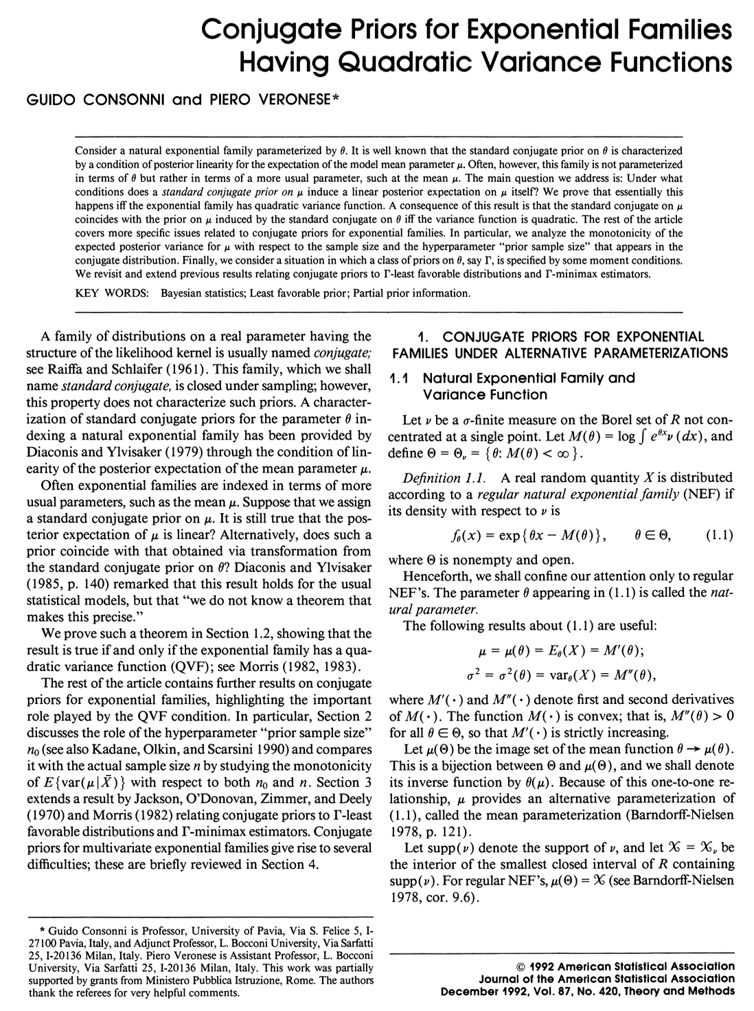
Consonni, G., and Veronese, P. (1992), “Conjugate priors for exponential families having quadratic functions,” Journal of the American Statistical Association, 87, 1123–1127.

Davison, A. C. (2003), Statistical Models, Cambridge University Press.

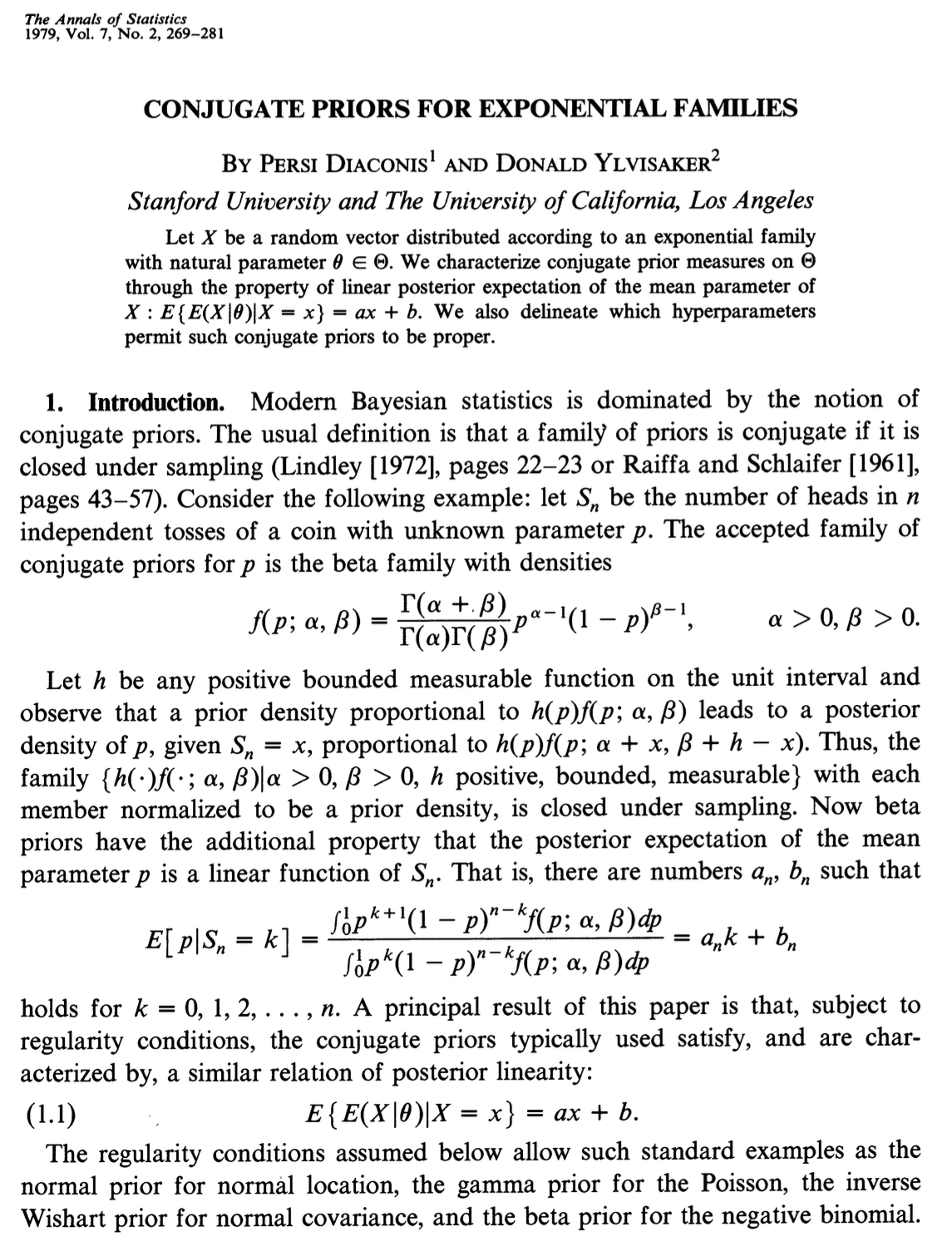
Diaconis, P., and Ylvisaker, D. (1979), “Conjugate prior for exponential families,” The Annals of Statistics, 7, 269–292.

Efron, B. (2023), Exponential Families in Theory and Practice, Cambridge University Press.

Efron, B., and Hastie, T. (2016), Computer Age Statistical Inference, Cambridge University Press.

Fisher, R. A. (1934), “Two new properties of mathematical likelihood,” Proceedings of the Royal Society of London. Series A, 144, 285–307.

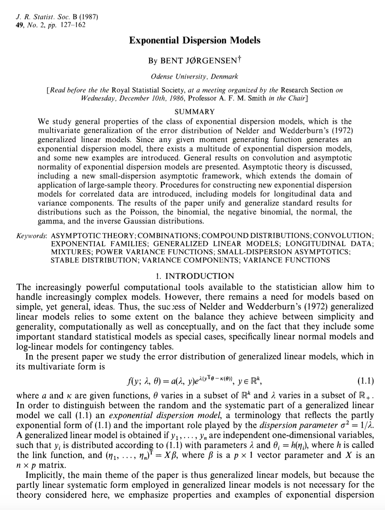
Jorgensen, B. (1987), “Exponential dispersion model,” Journal of the Royal Statistical Society. Series B: Methodological, 49, 127–162.

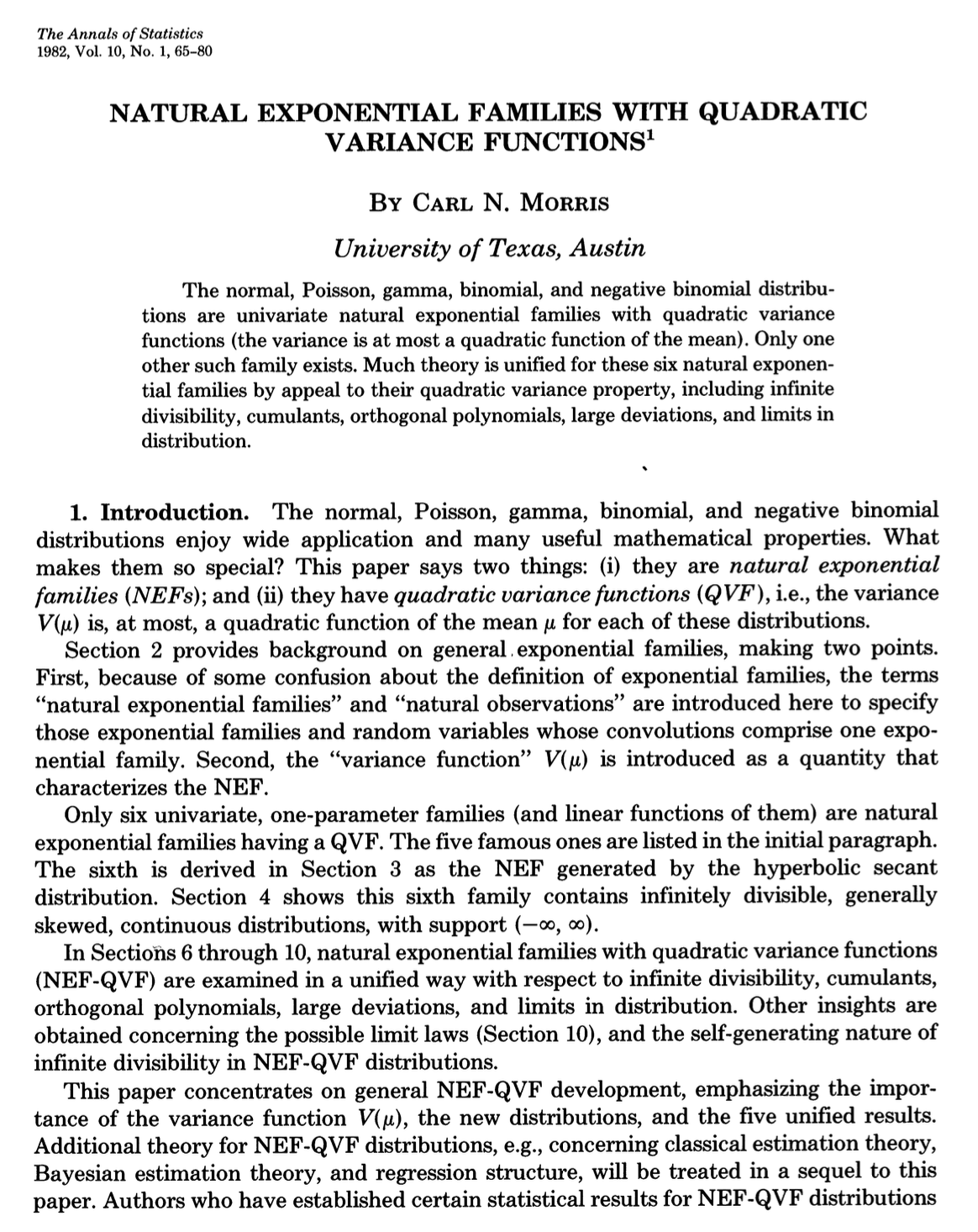
Morris, C. N. (1982), “Natural exponential families with quadratic variance functions,” Annals of Statistics, 10, 65–80.

Nelder, J. A., and Wedderburn, R. W. M. (1972), “Generalized linear models,” Journal of the Royal Statistical Society. Series A: Statistics in Society, 135, 370–384.

Pace, L., and Salvan, A. (1997), Principles of statistical inference from a Neo-Fisherian perspective, Advanced series on statistical science and applied probability, World Scientific.

Robert, C. P. (1994), The Bayesian Choice: from decision-theoretic foundations to computational implementation, Springer.