Optimism, Conflicts, and Trade-offs

Data Mining - CdL CLAMSES

Tommaso Rigon

Università degli Studi di Milano-Bicocca

Homepage

“Pluralitas non est ponenda sine necessitate.”

William of Ockham

• This unit will cover the following topics:

  • Bias-variance trade-off
  • Cross-validation
  • Information criteria
  • Optimism

• You may have seen these notions before…

• …but it is worth discussing the details of these ideas once again.

• They are indeed the foundations of statistical learning.

Yesterday’s and tomorrow’s data

Yesterday’s data

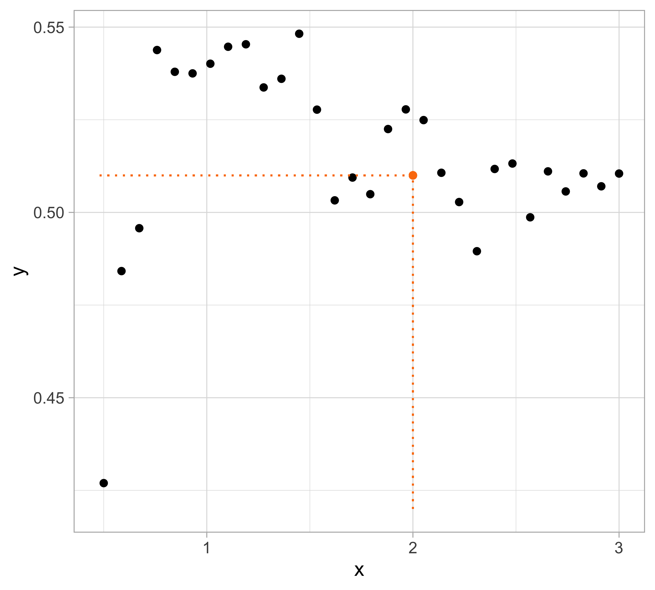
• Let us presume that yesterday we observed n = 30 pairs of data (x_i, y_i).

• Data were generated according to Y_i = f(x_i) + \epsilon_i, \quad i=1,\dots,n, with each y_i being the realization of Y_i.

• The \epsilon_1,\dots,\epsilon_n are iid “error” terms, such that \mathbb{E}(\epsilon_i)=0 and \text{var}(\epsilon_i)=\sigma^2 = 10^{-4}.

• Here f(x) is a regression function (signal) that we leave unspecified.

• Tomorrow we will get a new x. We wish to predict Y using \mathbb{E}(Y) = f(x).

Polynomial regression

• The function f(x) is unknown, therefore, it should be estimated.

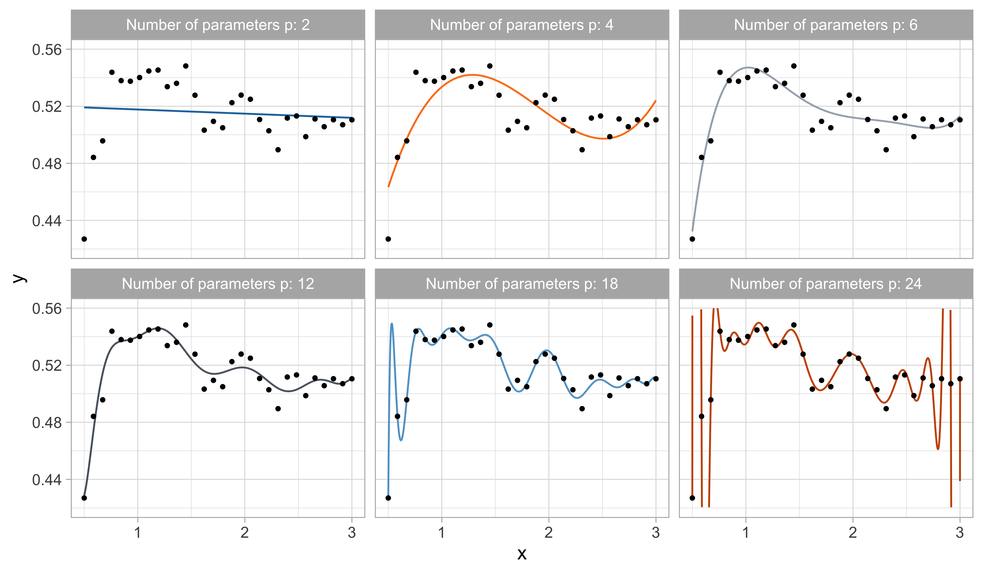
• A simple approach is using the tools of Unit A, such as polynomial regression: f(x; \beta) = \beta_1 + \beta_2 x + \beta_3 x^2 + \cdots + \beta_p x^{p-1}, namely f(x) is approximated with a polynomial of degree p-1 (i.e., Taylor expansions).

• This model is linear in the parameters: ordinary least squares can be applied.

• How do we choose the degree of the polynomial p - 1?

• Without clear guidance, in principle, any value of p \in \{1,\dots,n\} could be appropriate.

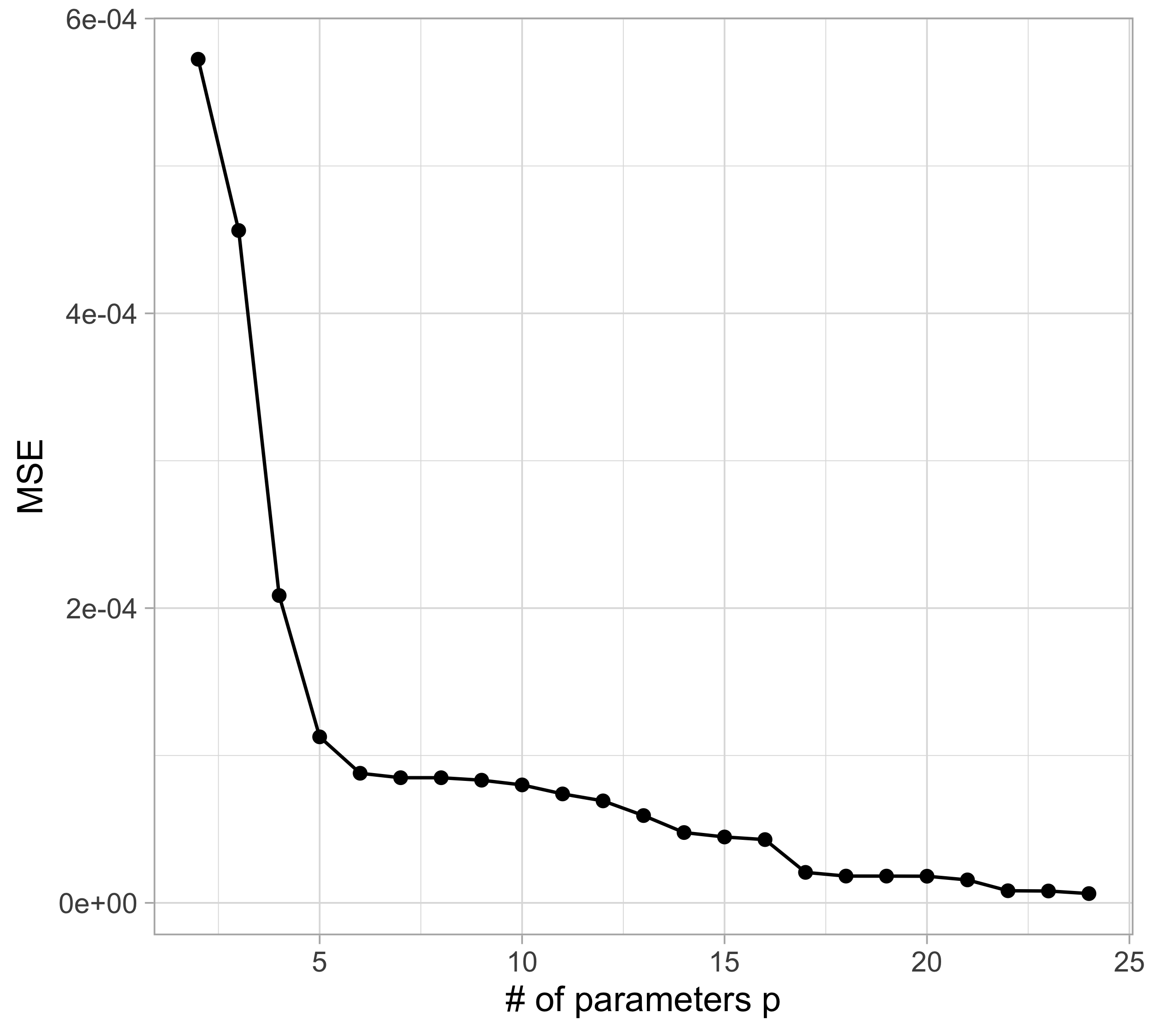
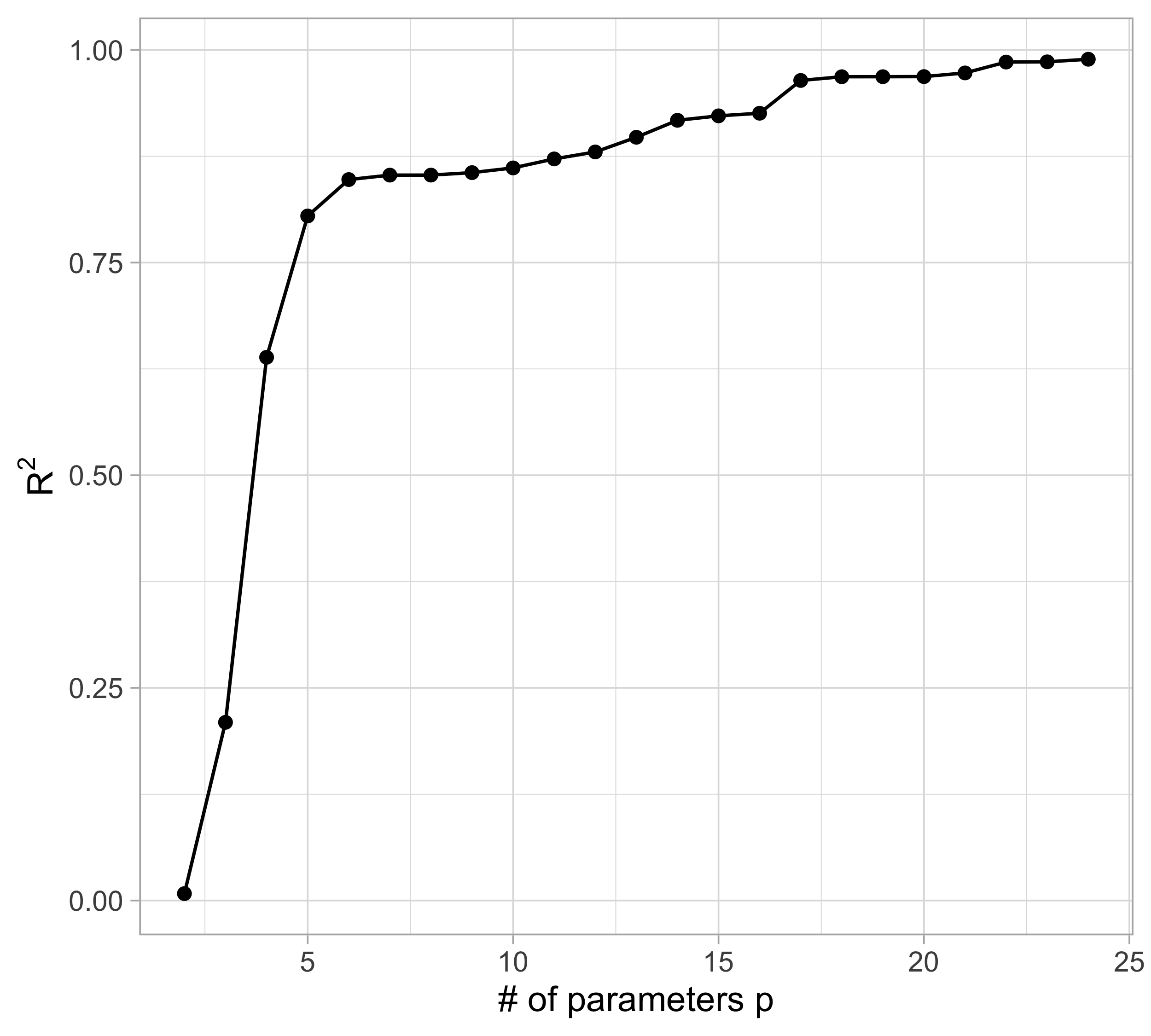
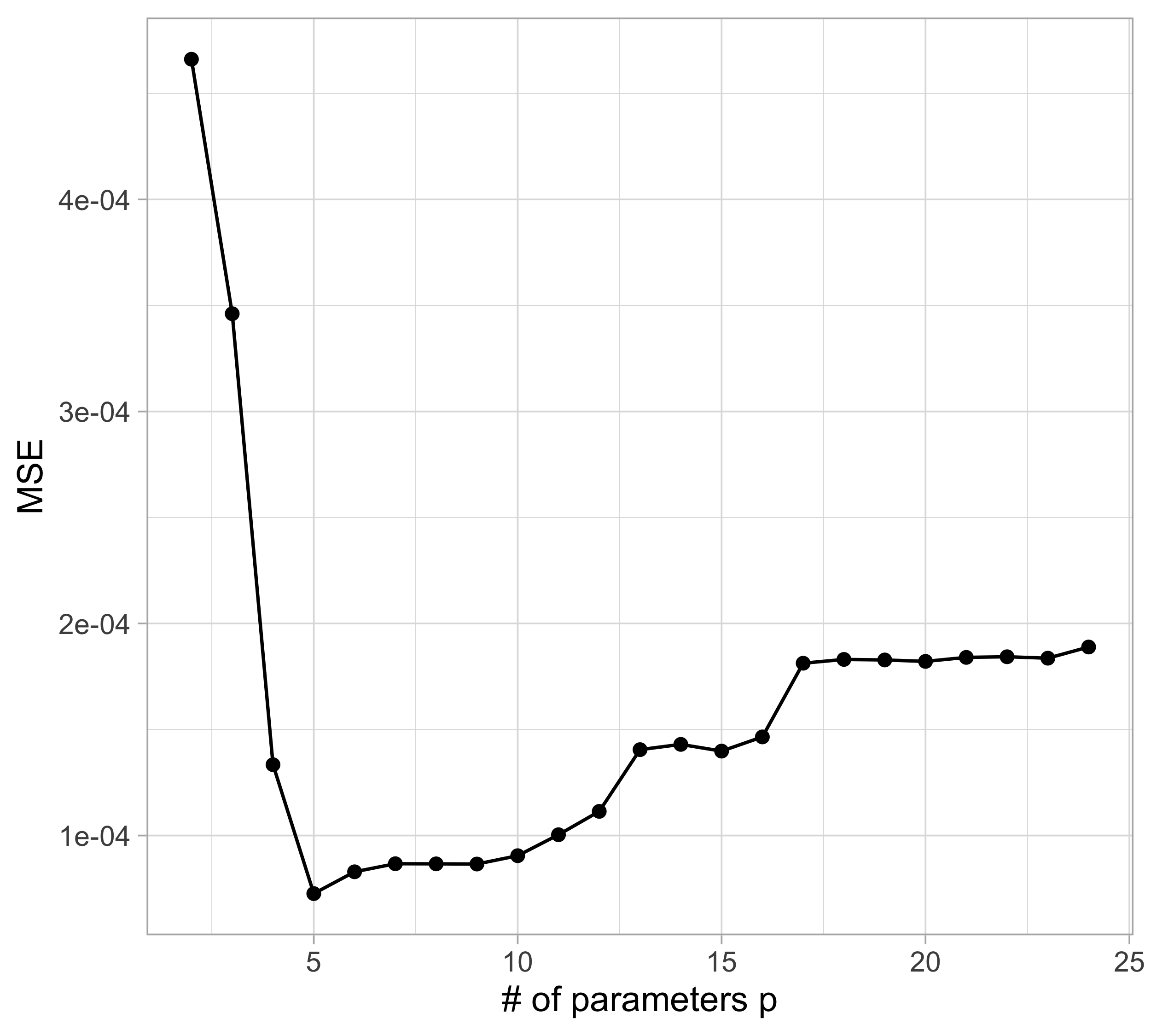
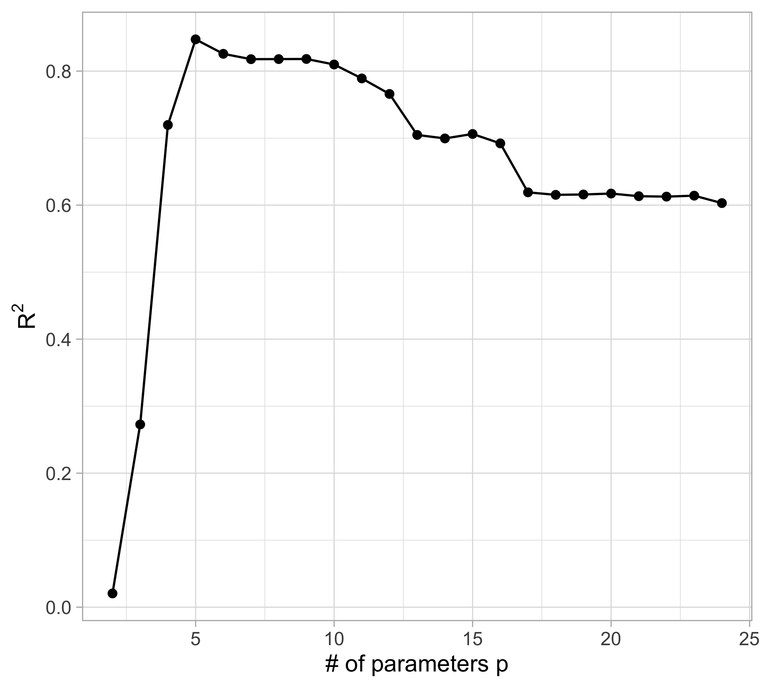
• Let us compare the mean squared error (MSE) on yesterday’s data (training) \text{MSE}_{\text{train}} = \frac{1}{n}\sum_{i=1}^n\{y_i -f(x_i; \hat{\beta})\}^2, or alternatively R^2_\text{train}, for different values of p…

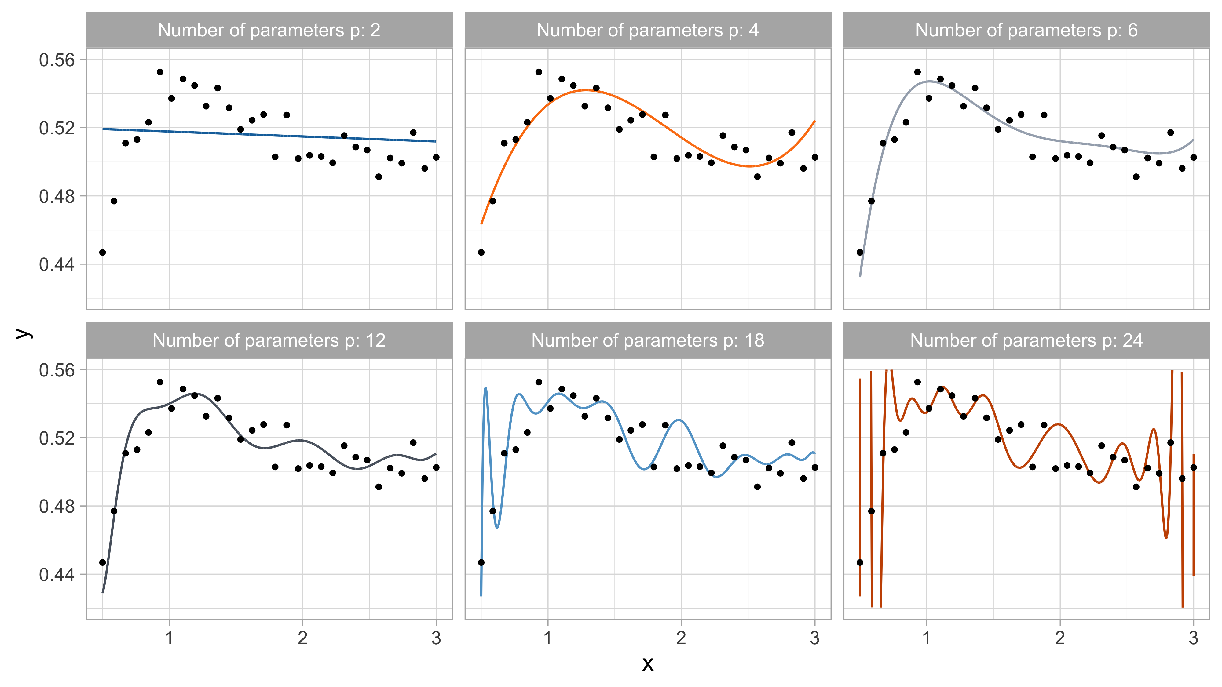
Yesterday’s data, polynomial regression

Yesterday’s data, goodness of fit

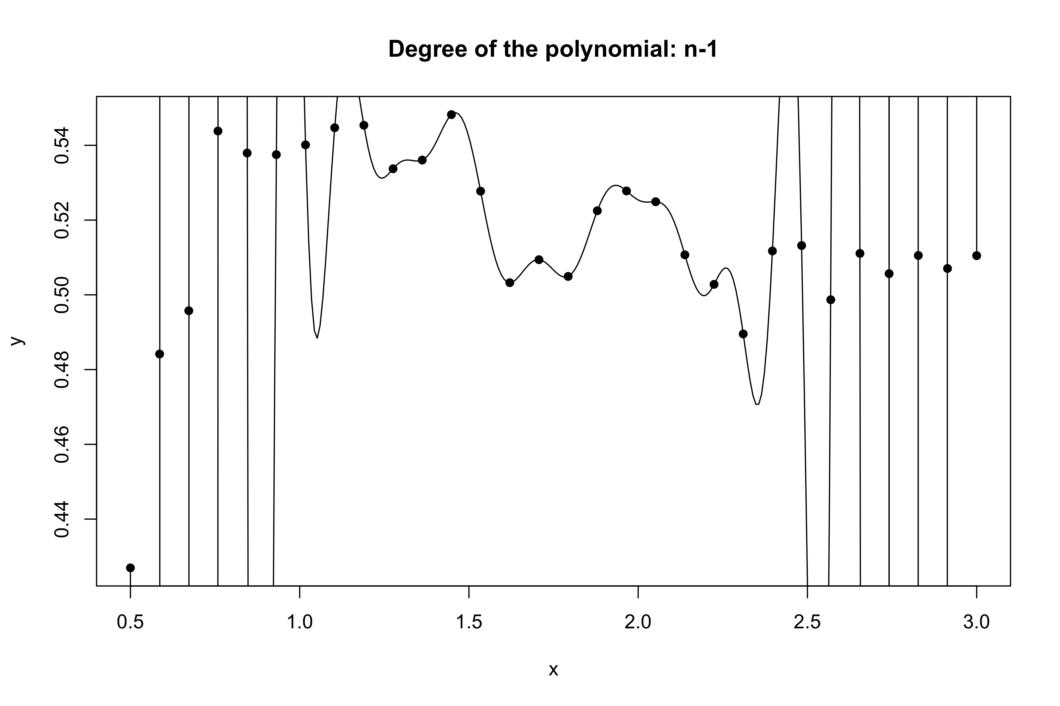
Yesterday’s data, polynomial interpolation (p = n)

Yesterday’s data, tomorrow’s prediction

• The MSE decreases as the number of parameter increases; similarly, the R^2 increases as a function of p. It can be proved that this always happens using ordinary least squares.

• One might be tempted to let p as large as possible to make the model more flexible…

• Taking this reasoning to the extreme would lead to the choice p = n, so that \text{MSE}_\text{train} = 0, \qquad R^2_\text{train} = 1, , i.e., a perfect fit. This procedure is called interpolation.

• However, we are not interested in predicting yesterday data. Our goal is to predict tomorrow’s data, i.e. a new set of n = 30 points: (x_1, \tilde{y}_1), \dots, (x_n, \tilde{y}_n), using \hat{y}_i = f(x_i; \hat{\beta}), where \hat{\beta} is obtained using yesterday’s data.

• Remark. Tomorrow’s r.v. \tilde{Y}_1,\dots, \tilde{Y}_n follow the same scheme as yesterday’s data.

Tomorrow’s data, polynomial regression

Tomorrow’s data, goodness of fit

Comments and remarks

• The mean squared error on tomorrow’s data (test) is defined as \text{MSE}_{\text{test}} = \frac{1}{n}\sum_{i=1}^n\{\tilde{y}_i -f(x_i; \hat{\beta})\}^2, and similarly the R^2_\text{test}. We would like the \text{MSE}_{\text{test}} to be as small as possible.

• For small values of p, an increase in the degree of the polynomial improves the fit. In other words, at the beginning, both the \text{MSE}_{\text{train}} and the \text{MSE}_{\text{test}} decrease.

• For larger values of p, the improvement gradually ceases, and the polynomial follows random fluctuations in yesterday’s data, which are not observed in the new sample.

• An over-adaptation to yesterday’s data is called overfitting, which occurs when the training \text{MSE}_{\text{train}} is low but the test \text{MSE}_{\text{test}} is high.

• Yesterday’s dataset is available from the textbook (A&S) website:

  • Dataset http://azzalini.stat.unipd.it/Book-DM/yesterday.dat
  • True f(\bm{x}) http://azzalini.stat.unipd.it/Book-DM/f_true.R

☠️ - Orthogonal polynomials

• When performing polynomial regression, the poly command computes an orthogonal basis of the original covariates (1, x, x^2,\dots,x^{p-1}) through the QR decomposition:

fit <- lm(y.yesterday ~ poly(x, degree = 3, raw = FALSE), data = dataset)
X <- model.matrix(fit)
colnames(X) = c("Intercept","x1","x2","x3")
round(t(X) %*% X, 8)

          Intercept x1 x2 x3
Intercept        30  0  0  0
x1                0  1  0  0
x2                0  0  1  0
x3                0  0  0  1

• Polynomial regression becomes numerically unstable when p \ge 13 (raw = TRUE, original polynomials) and p \ge 25 (raw = FALSE, orthogonal polynomials).

☠️ - Lagrange interpolating polynomials

• If the previous code does not work for p \ge 25, how was the plot of this slide computed?

• It turns out that for p = n there exists an alternative way of finding the ordinary least square solution, based on Lagrange interpolating polynomials, namely:

\hat{f}(x) = \sum_{i=1}^n\ell_i(x) y_i, \qquad \ell_i(x) = \prod_{k \neq i}\frac{x - x_k}{x_i - x_k}.

• Interpolating polynomials are clearly unsuitable for regression purposes, but may have interesting applications in other contexts.

Errors, trade-offs, and optimism

Summary and notation (fixed-X)

• In the previous example, we consider two sets of random variables:

  • The training set (yesterday) Y_1,\dots, Y_n, whose realization is y_1,\dots,y_n.
  • The test set (tomorrow) \tilde{Y}_1,\dots,\tilde{Y}_n, whose realization is \tilde{y}_1, \dots, \tilde{y}_n.

• The covariates \bm{x}_i = (x_{i1},\dots,x_{ip})^T in this scenario are deterministic. This is the so-called fixed-X design, which is a common assumption in regression models.

• We also assume that the random variables Y_i and \tilde{Y}_i are independent.

• In regression problems we customarily assume that Y_i = f(\bm{x}_i) + \epsilon_i, \qquad \tilde{Y}_i = f(\bm{x}_i) + \tilde{\epsilon}_i, \quad i=1,\dots,n, where \epsilon_i and \tilde{\epsilon}_i are iid “error” terms, with \mathbb{E}(\epsilon_i)=0 and \text{var}(\epsilon_i)=\sigma^2.

• In classification problems the relationship between \bm{x}_i and the Bernoulli r.v. Y_i \in \{0, 1\} is \mathbb{P}(Y_i = 1) = p(\bm{x}_i) = g\{f(\bm{x}_i)\}, \qquad i=1,\dots,n, where g(x) :\mathbb{R} \rightarrow (0,1) is monotone transformation, such as the inverse logit.

The in-sample prediction error

• The training data is used to estimate a function of the covariates \hat{f}(\bm{x}_i). We hope our predictions work well on the test set.

• A measure of quality for the predictions is the in-sample prediction error: \text{ErrF} = \mathbb{E}\left[\frac{1}{n} \sum_{i=1}^n \mathscr{L}\{\tilde{Y}_i; \hat{f}(\bm{x}_i)\}\right], where \mathscr{L}\{\tilde{Y}_i; \hat{f}(\bm{x}_i)\} is a loss function. The “F” is a reminder of the fixed-X design.

• The expectation is taken with respect to training random variable Y_1,\dots,Y_n, implicitly appearing in \hat{f}(\bm{x}), and the new data points \tilde{Y}_1,\dots,\tilde{Y}_n.

• The in-sample prediction error is measuring the average “discrepancy” between the new data points and the corresponding predictions based on the training.

Loss functions

• Examples of loss functions for regression problems Y \in \mathbb{R} are:

  • The quadratic loss \mathscr{L}\{\tilde{Y}_i; \hat{f}(\bm{x}_i)\} = \{\tilde{Y}_i - \hat{f}(\bm{x}_i)\}^2, leading to the MSE.
  • The absolute loss \mathscr{L}\{\tilde{Y}_i; \hat{f}(\bm{x}_i)\} = |\tilde{Y}_i - \hat{f}(\bm{x}_i)|, leading to the MAE.

• Examples of loss functions for binary classification problems Y \in \{0, 1\} are:

  • The misclassification loss, which is defined as \mathscr{L}\{\tilde{Y}_i; \hat{f}(\bm{x}_i)\} = \mathbb{I}(\tilde{Y}_i \neq \hat{y}_i). The predictions are obtained by dichotomizing the probabilities \hat{y}_i = \mathbb{I}(\hat{p}(\bm{x}_i) > 1/2).
  • The deviance or cross-entropy loss functions are defined as \mathscr{L}\{\tilde{Y}_i; \hat{f}(\bm{x}_i)\} = -2\left[ \mathbb{I}(Y_i = 1)\log{\hat{p}(\bm{x}_i)} + \mathbb{I}(Y_i = 0)\log{\{1 - \hat{p}(\bm{x}_i)}\}\right].

Regression under quadratic loss I

Error decomposition (reducible and irreducible)

In a regression problem, under a quadratic loss, each element of the in-sample prediction error admits the following decomposition \begin{aligned} \mathbb{E}\left[\{\tilde{Y}_i - \hat{f}(\bm{x}_i)\}^2\right] &= \mathbb{E}\left[\{f(\bm{x}_i) + \tilde{\epsilon}_i - \hat{f}(\bm{x}_i)\}^2\right] \\ & = \mathbb{E}\left[\{f(\bm{x}_i) - \hat{f}(\bm{x}_i)\}^2\right] + \mathbb{E}(\tilde{\epsilon}_i^2) + 2 \: \mathbb{E}\left[\tilde{\epsilon}_i \: \{f(\bm{x}_i) - \hat{f}(\bm{x}_i)\}\right]\\ & = \underbrace{\mathbb{E}\left[\{\hat{f}(\bm{x}_i) - f(\bm{x}_i)\}^2\right]}_{\text{reducible}} + \underbrace{\sigma^2}_{\text{irreducible}}, \end{aligned} recalling that \mathbb{E}(\tilde{\epsilon}_i^2) = \text{var}(\tilde{\epsilon}_i) = \sigma^2 and for any i = 1,\dots,n.

Regression under quadratic loss II

• We would like to make the mean squared error as small as possible, e.g., by choosing an “optimal” degree of the polynomial p-1 that minimizes it.

• Let us recall the previous decomposition \mathbb{E}\left[\{\tilde{Y}_i - \hat{f}(\bm{x}_i)\}^2\right] = \underbrace{\mathbb{E}\left[\{\hat{f}(\bm{x}_i) - f(\bm{x}_i)\}^2\right]}_{\text{reducible}} + \underbrace{\sigma^2}_{\text{irreducible}}, \quad i=1\dots,n.

• The best case scenario is when the estimated function coincides with the mean of \tilde{Y}_i, i.e.  \hat{f}(\bm{x}_i) = f(\bm{x}_i) = \mathbb{E}(\tilde{Y}_i), but even in this (overly optimistic) situation, we would still commit mistakes, due to the presence of \tilde{\epsilon}_i (unless \sigma^2 = 0). Hence, the variance \sigma^2 is called the irreducible error.

• Since we do not know f(\bm{x}_i), we seek for an estimate \hat{f}(\bm{x}_i) \approx f(\bm{x}_i), in the attempt of minimizing the reducible error.

Classification under misclassification loss

• In classification problems, under a misclassification loss, the in-sample prediction error is \text{ErrF} = \mathbb{E}\left[\frac{1}{n}\sum_{i=1}^n \mathscr{L}\{\tilde{Y}_i; \hat{f}(\bm{x}_i)\}\right] = \frac{1}{n}\sum_{i=1}^n \mathbb{E}\{\mathbb{I}(\tilde{Y}_i \neq \hat{y}_i)\}= \frac{1}{n}\sum_{i=1}^n\mathbb{P}(\tilde{Y}_i \neq \hat{y}_i).

• The above error is minimized whenever \hat{y}_i corresponds to Bayes classifier \hat{y}_{i, \text{bayes}} = \arg\max_{y \in \{0, 1\}} \mathbb{P}(\tilde{Y}_i = y) = \mathbb{I}(p(\bm{x}_i) > 0.5), which depends on the unknown probabilities p(\bm{x}_i).

• We call the Bayes rate the optimal in-sample prediction error: \mathbb{E}\left[\frac{1}{n}\sum_{i=1}^n \mathscr{L}\{\tilde{Y}_i; p(\bm{x}_i)\}\right] = \frac{1}{n}\sum_{i=1}^n\min\{p(\bm{x}_i), 1 - p(\bm{x}_i)\}.

• The Bayes rate is the error rate we would get if we knew the true p(\bm{x}) and can be regarded as the irreducible error for classification problems.

Bias-variance trade-off

• In many textbooks, including A&S, the starting point of the analysis is the reducible error, because it is the only one we can control and has a transparent interpretation.

• The reducible error measures the discrepancy between the unknown function f(\bm{x}) and its estimate \hat{f}(\bm{x}) and therefore it is a natural measure of the goodness of fit.

• What follows holds both for regression and classification problems.

Bias-variance decomposition

For any covariate value \bm{x}, it holds the following bias-variance decomposition: \mathbb{E}\left[\{\hat{f}(\bm{x}) - f(\bm{x})\}^2\right] = \underbrace{\mathbb{E}\left[\hat{f}(\bm{x}) - f(\bm{x})\right]^2}_{\text{Bias}^2} + \underbrace{\text{var}\{\hat{f}(\bm{x})\}}_{\text{variance}}.

Example: bias-variance in linear regression models

• In regression problems the in-sample prediction error under squared loss is \begin{aligned} \text{ErrF} = \sigma^2 + \frac{1}{n}\sum_{i=1}^n\mathbb{E}\left[\hat{f}(\bm{x}_i) - f(\bm{x}_i)\right]^2 + \frac{1}{n}\sum_{i=1}^n\text{var}\{\hat{f}(\bm{x}_i)\}. \end{aligned}

• In ordinary least squares the above quantity can be computed in closed form, since each element of the bias term equals \mathbb{E}\left[f(\bm{x}_i; \hat{\beta}) - f(\bm{x}_i)\right] = \bm{x}_i^T(\bm{X}^T\bm{X})^{-1}\bm{X}^T\bm{f} - f(\bm{x}_i). where \bm{f} = (f(\bm{x}_1),\dots,f(\bm{x}_n))^T. Note that if f(\bm{x}) = \bm{x}^T\beta, then the bias is zero.

• Moreover, in ordinary least squares the variance term equals \frac{1}{n}\sum_{i=1}^n\text{var}\{f(\bm{x}_i; \hat{\beta})\} = \frac{\sigma^2}{n}\sum_{i=1}^n \bm{x}_i^T (\bm{X}^T\bm{X})^{-1}\bm{x}_i = \frac{\sigma^2}{n}\text{tr}(\bm{H}) = \sigma^2 \frac{p}{n}.

If we knew f(x)…

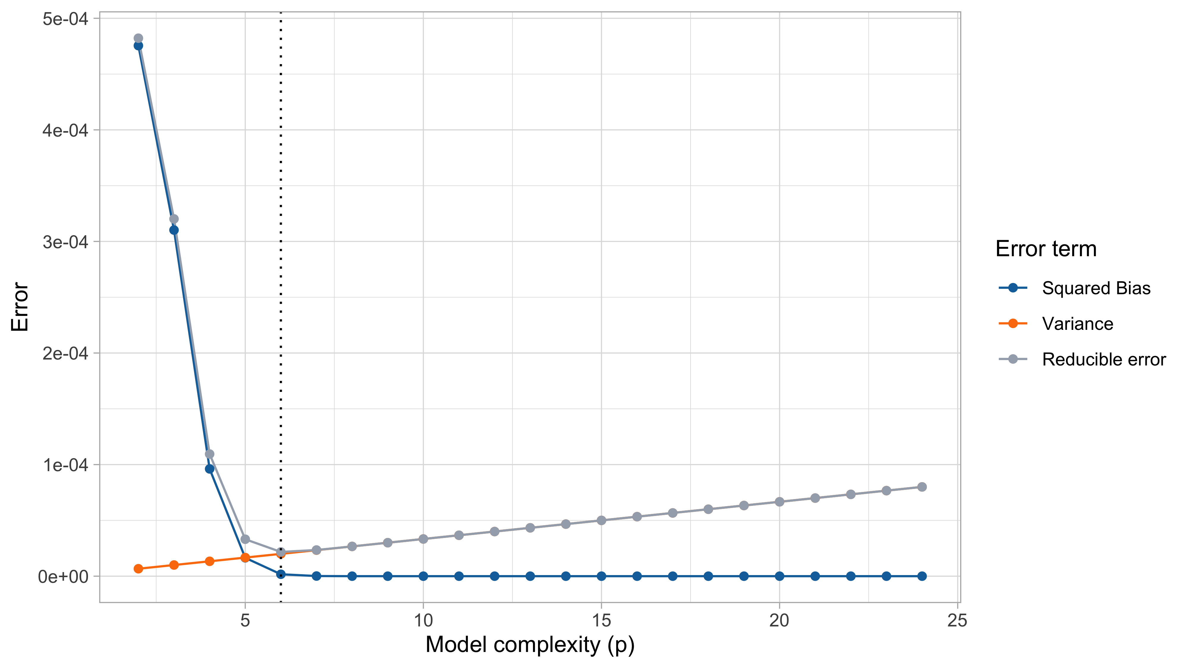
Bias-variance trade-off

• When p grows, the mean squared error first decreases and then it increases. In the example, the theoretical optimum is p = 6 (5th degree polynomial).

• The bias measures the ability of \hat{f}(\bm{x}) to reconstruct the true f(\bm{x}). The bias is due to lack of knowledge of the data-generating mechanism. It equals zero when \mathbb{E}\{\hat{f}(\bm{x})\} = f(\bm{x}).

• The bias term can be reduced by increasing the flexibility of the model (e.g., by considering a high value for p).

• The variance measures the variability of the estimator \hat{f}(\bm{x}) and its tendency to follow random fluctuations of the data.

• The variance increases with the model complexity.

• It is not possible to minimize both the bias and the variance, there is a trade-off.

• We say that an estimator is overfitting the data if an increase in variance comes without important gains in terms of bias.

But since we do not know f(x)…

• We just concluded that we must expect a trade-off between error and variance components. In practice, however, we cannot do this because, of course, f(x) is unknown.

• A simple solution consists indeed in splitting the observations in two parts: a training set (y_1,\dots,y_n) and a test set (\tilde{y}_1,\dots,\tilde{y}_n), having the same covariates x_1,\dots,x_n.

• We fit the model \hat{f} using n observations of the training and we use it to predict the n observations on the test set.

• This leads to an unbiased estimate of the in-sample prediction error, i.e.: \widehat{\mathrm{ErrF}} = \frac{1}{n}\sum_{i=1}^n\mathscr{L}\{\tilde{y}_i; \hat{f}(\bm{x}_i)\}.

• This is precisely what we already did with yesterday’s and tomorrow’s data!

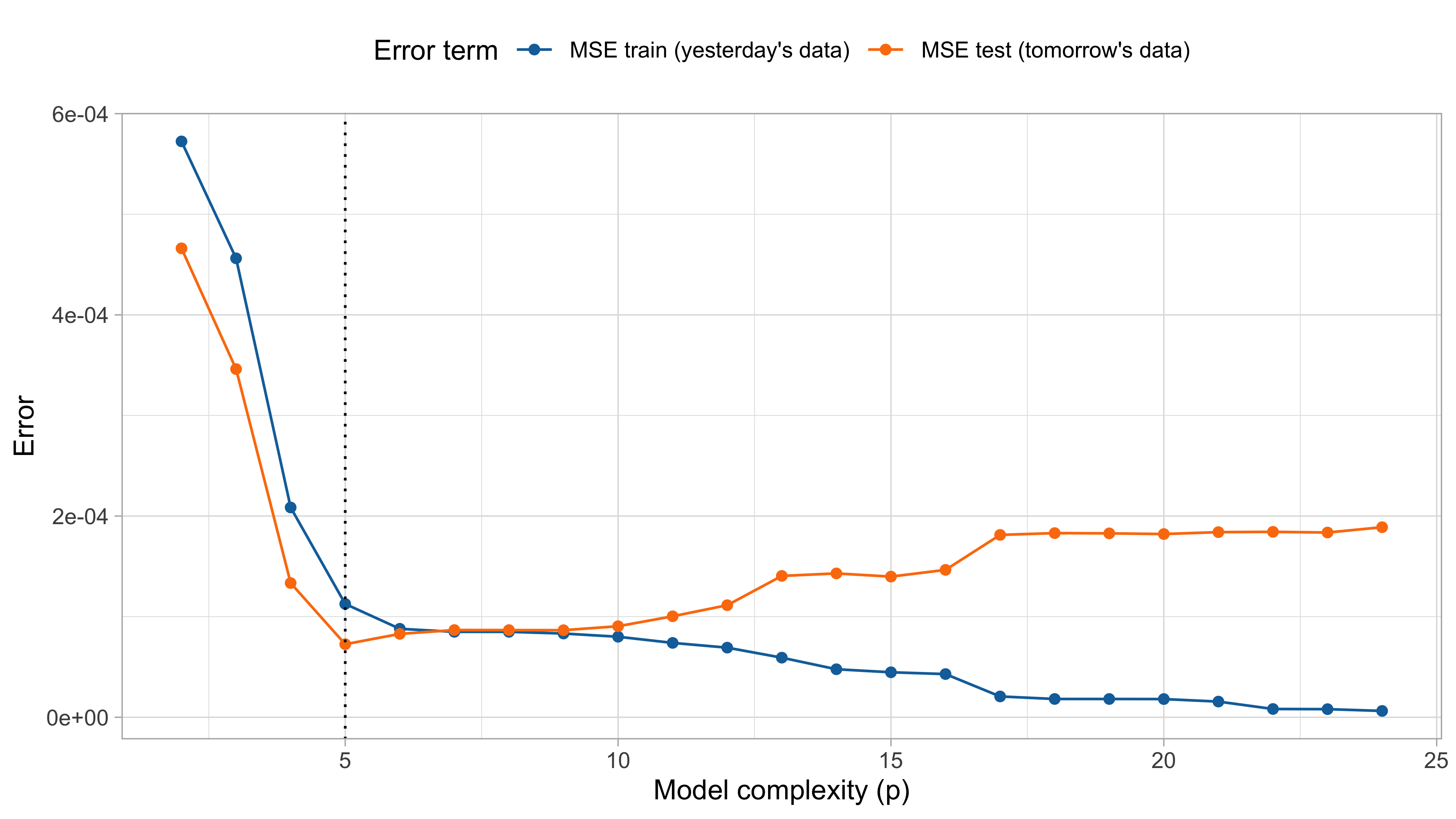
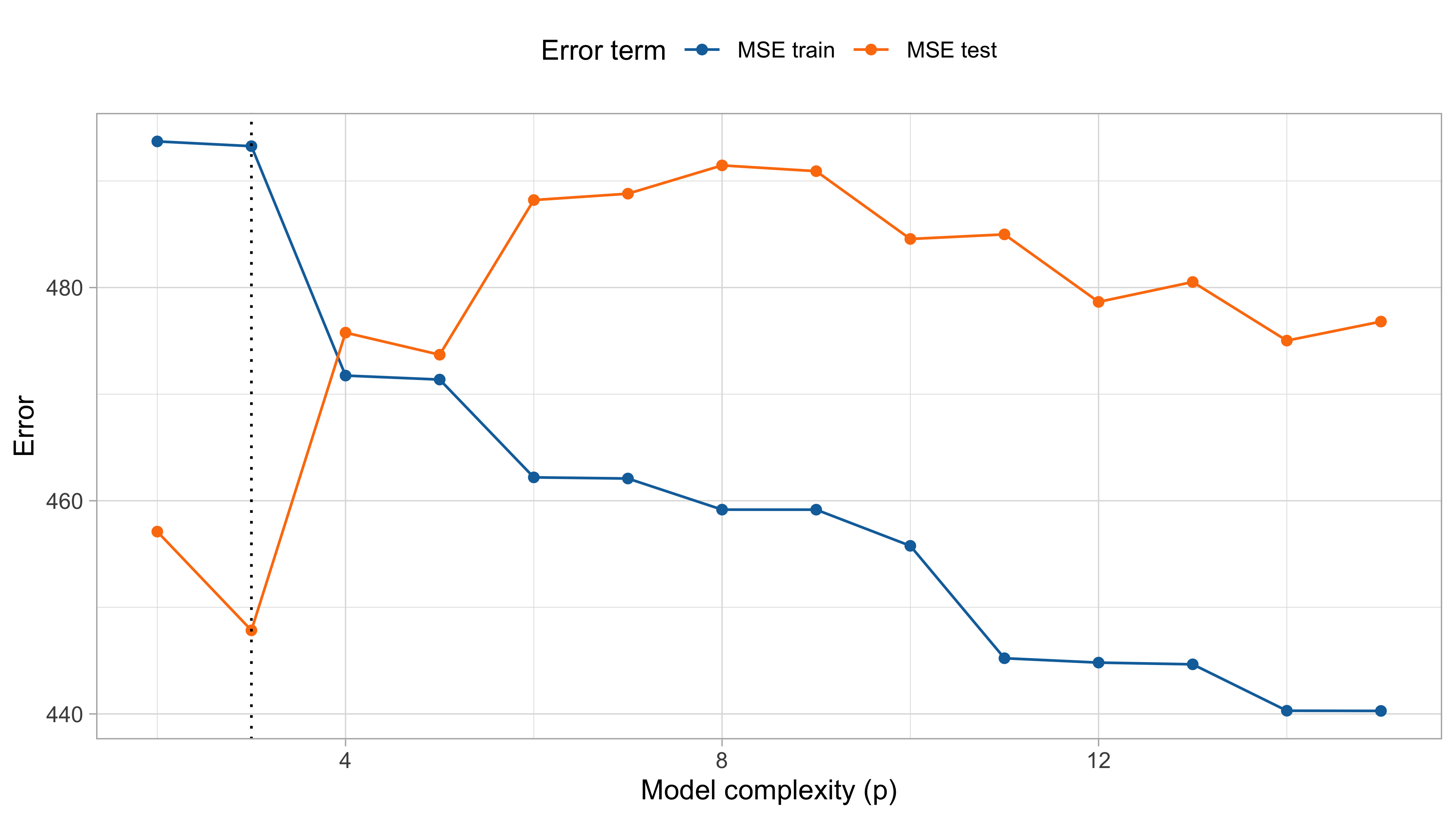
MSE on training and test set (recap)

Optimism I

• Let us investigate this discrepancy between training and test more in-depth.

• In regression problems, under a squared loss function, the in-sample prediction error is \text{ErrF} = \mathbb{E}(\text{MSE}_\text{test}) = \frac{1}{n}\sum_{i=1}^n\mathbb{E}\left[\{\tilde{Y}_i - \hat{f}(\bm{x}_i)\}^2\right]

• Similarly, the in-sample training error can be defined as follows \mathbb{E}(\text{MSE}_\text{train}) = \frac{1}{n}\sum_{i=1}^n\mathbb{E}\left[\{Y_i - \hat{f}(\bm{x}_i)\}^2\right].

• We already know that \mathbb{E}(\text{MSE}_\text{train}) provides a very optimistic assessment of the model performance. For example when p = n then \mathbb{E}(\text{MSE}_\text{train}) = 0.

• We call optimism the difference between these two quantities: \text{Opt} = \mathbb{E}(\text{MSE}_\text{test}) - \mathbb{E}(\text{MSE}_\text{train}).

Optimism II

• It can be proved (see Exercises) that the optimism has a very simple form: \text{Opt} = \frac{2}{n}\sum_{i=1}^n\text{cov}(Y_i, \hat{f}(\bm{x}_i))

• If ordinary least squares are employed, then the predictions are \bm{H}\bm{Y}, therefore \text{Opt}_\text{ols} = \frac{2}{n} \text{tr}\{\text{cov}(\bm{Y}, \bm{H}\bm{Y})\} = \frac{2}{n} \text{tr}\{\text{cov}(\bm{Y}, \bm{Y}) \bm{H}^T\} = \frac{2 \sigma^2}{n}\text{tr} (\bm{H}) = \frac{2 \sigma^2 p}{n}.

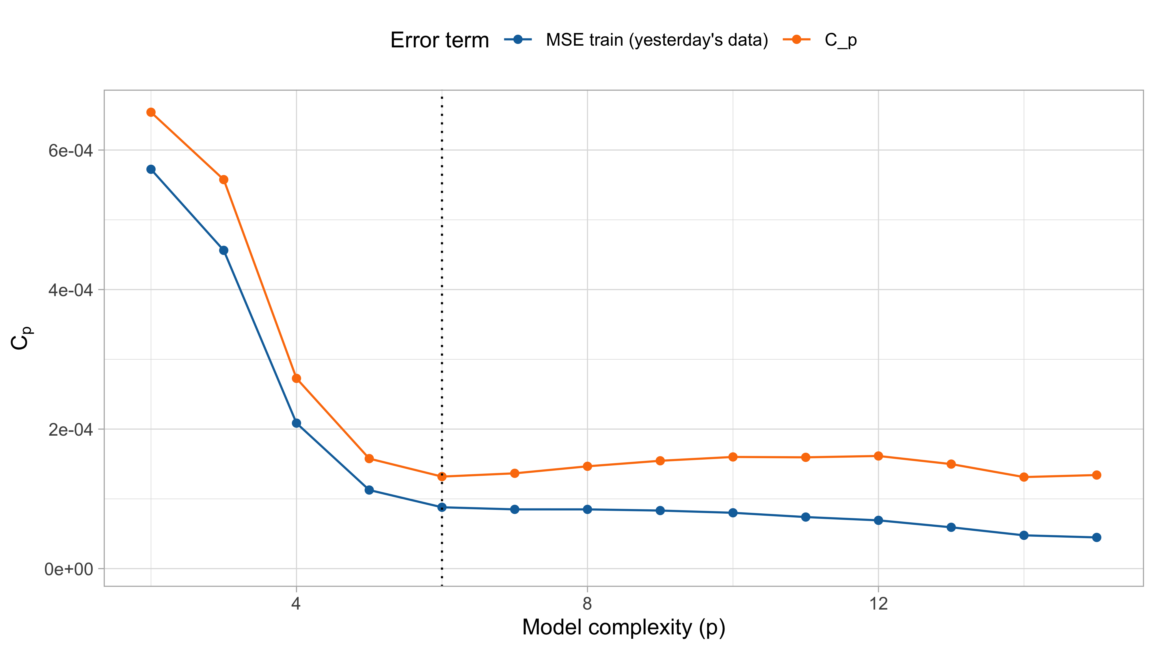
• This leads to an estimate for the in-sample prediction error, known as C_p of Mallows: \widehat{\mathrm{ErrF}} = \text{MSE}_\text{train} + \text{Opt}_\text{ols} = \frac{1}{n}\sum_{i=1}^n\{y_i - f(\bm{x}_i; \hat{\beta})\}^2 + \frac{2 \sigma^2 p}{n}.

• If \sigma^2 is unknown, then it must be estimated using for instance s^2.

Optimism III

Cross-validation

Another example: cholesterol data

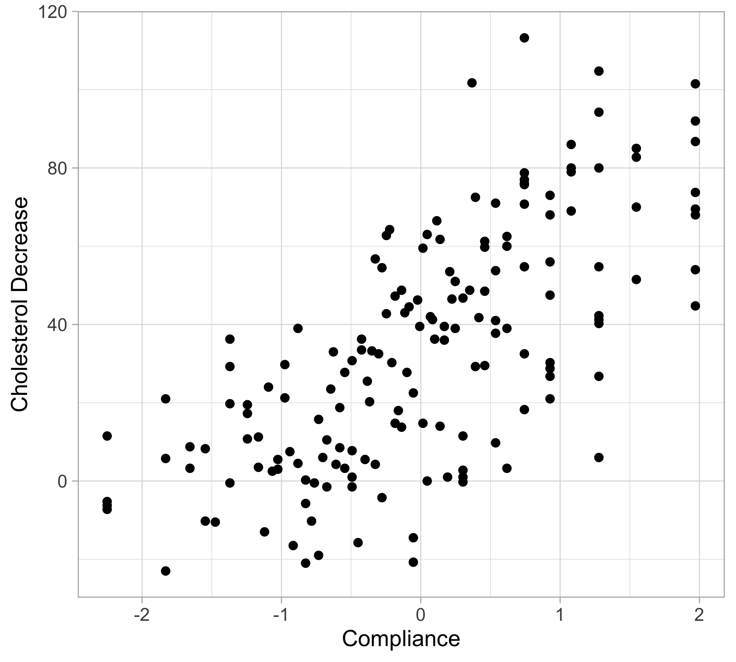
• A drug called “cholestyramine” is administered to n = 164 men.

• We observe the pair (x_i, y_i) for each man.

• The response y_i is the decrease in cholesterol level over the experiment.

• The covariate x_i is a measure of compliance.

• We assume, as before, that the data are generated according to Y_i = f(x_i) + \epsilon_i, \quad i=1,\dots,n.

• The original data can be found here.

Summary and notation (random-X)

• A slight change to the previous setup is necessary. In fact, there are no reasons to believe that the compliance is a fixed covariate.

• We consider a set of iid random variables (X_1, Y_1),\dots, (X_n, Y_n), whose realization is (\bm{x}_1,y_1),\dots,(\bm{x}_n, y_n). This time, the covariates are random.

• The main assumption is that these pairs are iid, namely: (X_i, Y_i) \overset{\text{iid}}{\sim} \mathcal{P}, \quad i=1,\dots,n.

• Conditionally on X_i = \bm{x}_i, in regression problems we let as before Y_i = f(\bm{x}_i) + \epsilon_i, \quad i=1,\dots,n, where \epsilon_i are iid “error” terms with \mathbb{E}(\epsilon_i)=0 and \text{var}(\epsilon_i)=\sigma^2.

Expected prediction error

• In this setting with random covariates, we want to minimize the expected prediction error: \text{Err} = \mathbb{E}\left[\mathscr{L}\{\tilde{Y}; \hat{f}(\tilde{X})\}\right], where (\tilde{X},\tilde{Y}) \sim \mathcal{P} is a new data point and \hat{f} is an estimate using n observations.

• We can randomly split the original set of data \{1,\dots,n\} into two groups V_\text{train} and V_\text{test}.

• We call \hat{f}_\text{train} the estimate based on the data in V_\text{train}.

• Then, we obtain a (slightly biased) estimate of \text{Err} by using the empirical quantity: \widehat{\mathrm{Err}} = \frac{1}{|V_\text{test}|}\sum_{i \in V_\text{test}}\mathscr{L}\{\tilde{y}_i; \hat{f}_\text{train}(\bm{x}_i)\}.

• The data-splitting strategy we used before is an effective tool for assessing the error. However, its interpretation is changed: we are now estimating \text{Err} and not \text{ErrF}.

MSE on training and test (cholesterol data)

Training, validation, and test I

• On many occasions, we may need to select several complexity parameters and compare hundreds of models.

• If the same test set is used for such a task, the final assessment of the error is somewhat biased and too optimistic, because we are “learning” from the test set.

• If we are in a data-rich situation, the best approach is to divide the dataset into three parts randomly:

  • a training set, used for fitting the models;
  • a validation set, used to estimate prediction error and perform model selection;
  • a test set, for assessment of the error of the final chosen model.

• Ideally, the test set should be kept in a “vault” and be brought out only at the end of the data analysis.

Training, validation, and test II

• There is no precise rule on how to select the size of these sets; a rule of thumb is given in the picture below.

• The training, validation, and test setup reduces the number of observations we can use to fit the models. It could be problematic if the sample size is relatively small.

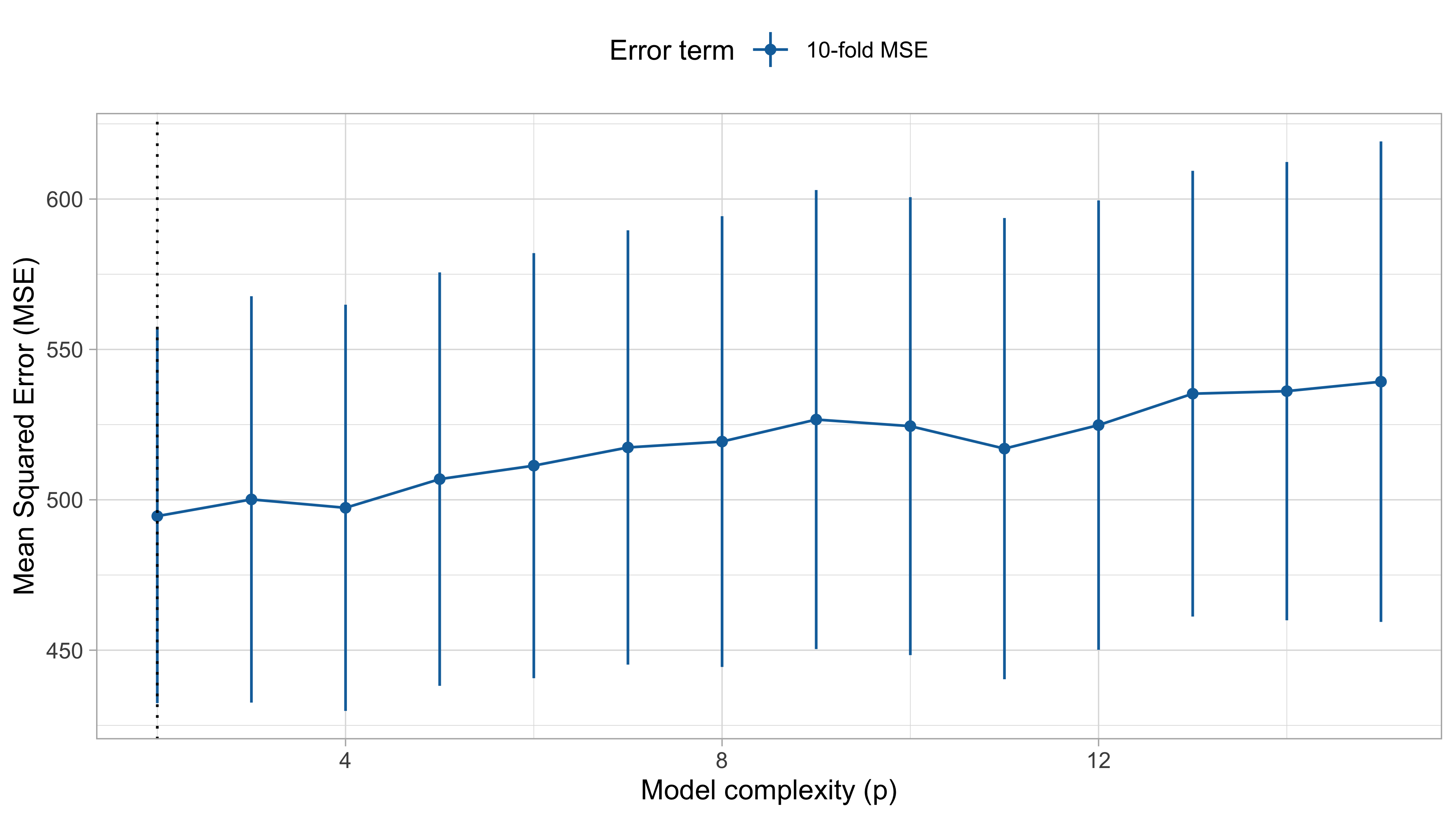
Cross-validation I

• A way to partially overcome the loss of efficiency of the training / test paradigm consists in randomly splitting the data \{1,\dots,n\} in equal parts, say V_1,\ldots,V_K.

• In the K-fold cross-validation method we use the observations i \notin V_k to train the model and the remaining observations i \in V_k to perform model selection.

• In the following scheme, we let K = 5.

Cross-validation II

• In the K-fold cross validation we compute for each fold k we fit a model \hat{f}_{-V_k}(\bm{x}) without using the observations of V_k.

• Hence, the model must be estimated K times, which could be computationally challenging.

• The error of each on the kth folds is computed as \widehat{\text{Err}}_{V_k} = \frac{1}{|V_k|} \sum_{i \in V_k} \mathscr{L}\{y_i; \hat{f}_{-V_k}(\bm{x}_i)\}, where |V_k| is the cardinality of V_k, i.e. V_k \approx n / K.

• We summarize the above errors using the mean, obtaining the following estimate for the expected prediction error: \widehat{\mathrm{Err}} = \frac{1}{K} \sum_{k=1}^{K} \widehat{\text{Err}}_{V_k}= \frac{1}{K} \sum_{k=1}^{K}\left[ \frac{1}{|V_k|} \sum_{i \in V_k} \mathscr{L}\{y_i; \hat{f}_{-V_k}(\bm{x}_i)\} \right].

Cross-validation III

• An advantage of CV is that variance of the Monte Carlo estimate \widehat{\mathrm{Err}} can be quantified.

• Let us define cross-validated “residuals” of our procedure as follows r_i = \mathscr{L}\{y_i; \hat{f}_{-V_k}(\bm{x}_i)\}, \qquad i=1,\dots,n. so that \widehat{\text{Err}} = \bar{r}. Does it coincide with the estimate \widehat{\text{Err}} presented in the previous slide? Recall that V_k \approx n / K…

• Then, a simple estimate for the standard error of \widehat{\text{Err}} is \widehat{\text{se}} = \frac{1}{\sqrt{n}} \text{sd}(r) = \frac{1}{\sqrt{n}} \sqrt{\frac{1}{n-1}\sum_{i=1}^n (r_i - \bar{r})^2}.

• The above formula is often criticized for producing intervals that are too narrow!

• Indeed, the estimate \widehat{\text{se}} of the standard deviation of \widehat{\text{Err}} assumes that the observed errors r_1, \dots, r_n are independent, but this is false!

Cross-validation IV (cholesterol data)

Leave-one-out cross-validation

• The maximum possible value for K is n, the leave-one-out cross-validation (LOO-CV).

• The LOO-CV is hard to implement because it requires the estimation of n different models.

• However, in ordinary least squares there is a brilliant computational shortcut.

LOO-CV (Ordinary least squares)

Let \hat{y}_{-i} = \bm{x}_i^T\hat{\beta}_{-i} be the leave-one-out predictions of a linear model and let h_i = [\bm{H}]_{ii} and \hat{y}_i be the leverages and the predictions of the full model. Then: y_i - \hat{y}_{-i} = \frac{y_i - \hat{y}_i}{1 - h_i}, \qquad i=1,\dots,n. Therefore, the leave-one-out mean squared error is \widehat{\mathrm{Err}} = \frac{1}{n} \sum_{i=1}^{n} \widehat{\text{Err}}_{V_i}= \frac{1}{n}\sum_{i=1}^n \left(\frac{y_i - \hat{y}_i}{1 - h_i}\right)^2.

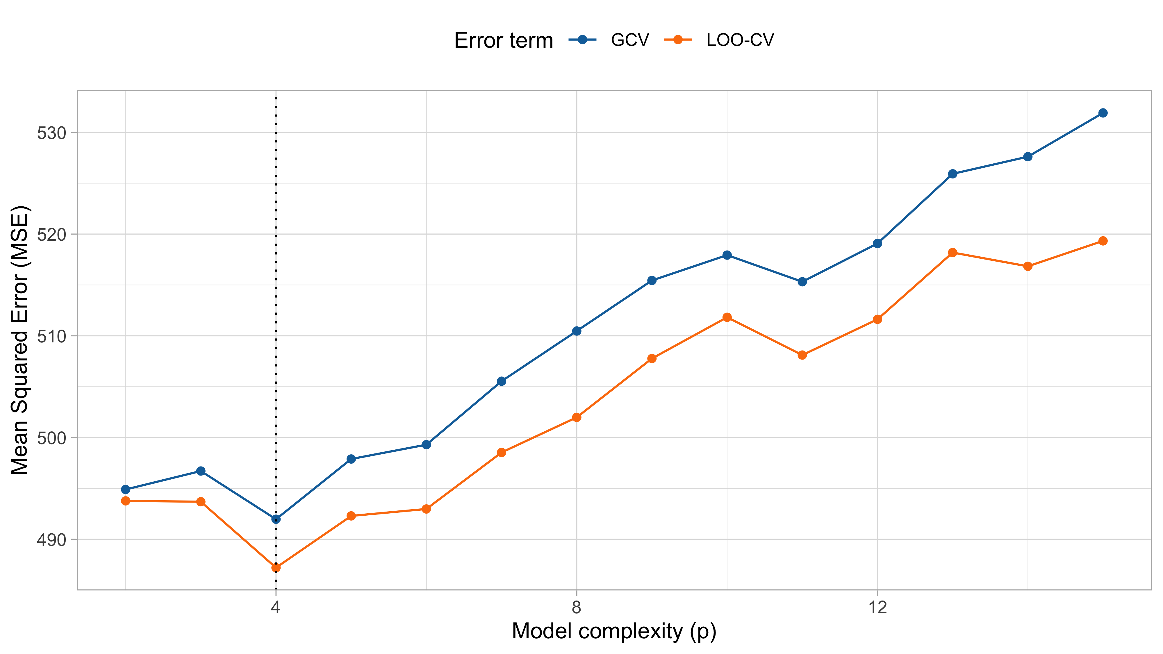
Generalized cross-validation

• An alternative to LOO-CV is the so-called generalized cross validation (GCV), defined as \text{GCV} = \widehat{\mathrm{Err}} = \frac{1}{n}\sum_{i=1}^n \left(\frac{y_i - \hat{y}_i}{1 - p/n}\right)^2.
• The GCV is an approximate LOO-CV for ordinary least squares, in which the leverages h_i are replaced by their mean: \frac{1}{n}\sum_{i=1}^n h_i = \frac{p}{n}.
• For small x >0 it holds that (1 - x)^{-2} \approx 1 + 2x. Then, we will write \text{GCV} \approx \frac{1}{n}\sum_{i=1}^n\{y_i - f(\bm{x}_i; \hat{\beta})\}^2 + \frac{2\hat{\sigma}^2 p}{n}, \qquad \hat{\sigma}^2 =\frac{1}{n}\sum_{i=1}^n\{y_i - f(\bm{x}_i; \hat{\beta})\}^2, revealing a sharp connection with the C_p of Mallows.

LOO-CV and GCV (cholesterol data)

On the choice of K

• Common choices are K = 5 or K = 10. It is quite evident that a larger K requires more computations.

• A K-fold CV with K=5 or K = 10 is a (upwords) biased estimate of \text{Err} because it uses less observations than those available (either 4/5 or 9/10).

• The LOO-CV has a very small bias, since each fit uses n-1 observations, but it has high variance, being the average of n highly positively correlated quantities.

• Indeed, the estimates \hat{f}_{-i} and \hat{f}_{-i'} have n - 2 observations in common. Recall that the variance of the sum is: \text{var}(X + Y) = \text{var}(X) + \text{var}(Y) + 2\text{cov}(X, Y).

• Overall, the choice is very much context-dependent.

Information criteria

Goodness of fit with a penalty term

• The main statistical method for estimating unknown parameters of a model is the maximize the log-likelihood \ell(\theta) = \ell(\theta; y_1,\dots,y_n).

• However, we cannot pick the value of p that maximizes the log-likelihood (why not?)

• We must consider the different number of parameters, introducing a penalty: \text{IC}(p) = -2 \ell(\hat{\theta}) + \text{penalty}(p),

• The \text{IC} is called an information criterion. We select the number of parameters minimizing the \text{IC}.

• The choice of the specific penalty identifies a particular criterion.

• An advantage of \text{IC} is that they are based on the full dataset.

The Akaike information criterion I

• Akaike suggested minimizing over p the expectation of the Kullback-Leibler divergence: \text{KL}(p(\cdot; \theta_0) \mid\mid p(\cdot;\hat{\theta})) = \int p(\tilde{\bm{Y}};\theta_0) \log{p(\tilde{\bm{Y}};\theta_0)}\mathrm{d}\tilde{\bm{Y}} - \int p(\tilde{\bm{Y}};\theta_0)\log{p(\tilde{\bm{Y}};\hat{\theta})\mathrm{d}\tilde{\bm{Y}}}, between the “true” model p(\bm{Y};\theta_0) with parameter \theta_0 and the estimated model p(\bm{Y};\hat{\theta}).

• In the above Kullback-Leibler, for any fixed p, the parameter \theta is replaced with its maximum likelihood estimator \hat{\theta} = \hat{\theta}(\bm{Y}), using the data \bm{Y} = (Y_1,\dots,Y_n).

• Equivalently, we can select p such that the expectation w.r.t. p(\bm{Y}; \theta_0) \begin{aligned} \Delta(p) &= 2 \: \mathbb{E}_{\theta_0}\left[\text{KL}(p(\cdot; \theta_0) \mid\mid p(\cdot;\hat{\theta}))\right] - \underbrace{2 \int p(\tilde{\bm{Y}};\theta_0) \log{p(\tilde{\bm{Y}};\theta_0)}\mathrm{d}\tilde{\bm{Y}}}_{\text{Does not depend on } p} \\ & = - 2 \: \mathbb{E}_{\theta_0}\left[\int p(\tilde{\bm{Y}};\theta_0)\log{p(\tilde{\bm{Y}};\hat{\theta})\mathrm{d}\tilde{\bm{Y}}} \right] \end{aligned} is minimized. Unfortunately, we cannot compute nor minimize \Delta(p) because \theta_0 is unknown.

The Akaike information criterion II

• The theoretical quantity \Delta(p) cannot be obtained. However, the quantity \text{AIC} = -2 \ell(\hat{\theta}) + 2 p, namely the Akaike information criterion, is a good estimator of \Delta(p).

• More formally, it can be proved that under technical conditions: \mathbb{E}_{\theta_0}(\text{AIC}) + o(1) = \Delta(p), for n \rightarrow \infty.

• In practice, we will select the value of p minimizing the \text{AIC}, which is typically quite easy.

• The factor 2 is just a convention, introduced to match the quantities of the usual asymptotic theory.

The AIC for Gaussian linear models

• Let us assume that \sigma^2 is known. Then the \text{AIC} for a Gaussian linear model is \begin{aligned} \text{AIC} &= -2 \ell(\hat{\beta}) + 2 p = -2 \left\{-\frac{n}{2}\log{(2\pi\sigma^2)} - \frac{1}{2 \sigma^2}\sum_{i=1}^n (y_i - \bm{x}_i^T\hat{\beta})^2\right\} + 2p \\ & = n\log{(2\pi\sigma^2)} + \frac{n}{ \sigma^2}\left\{ \frac{1}{n}\sum_{i=1}^n (y_i - \bm{x}_i^T\hat{\beta})^2 + \frac{2p\sigma^2}{n} \right\} \\ & = n\log{(2\pi\sigma^2)} + \frac{n}{ \sigma^2} C_p, \end{aligned} implying that for fixed values \sigma^2 the C_p of Mallows and the Akaike’s \text{AIC} are equivalent, i.e. they lead to the same minimum.

• When \sigma^2 is unknown, then it is estimated, and the C_p and \text{AIC} may be slightly different.

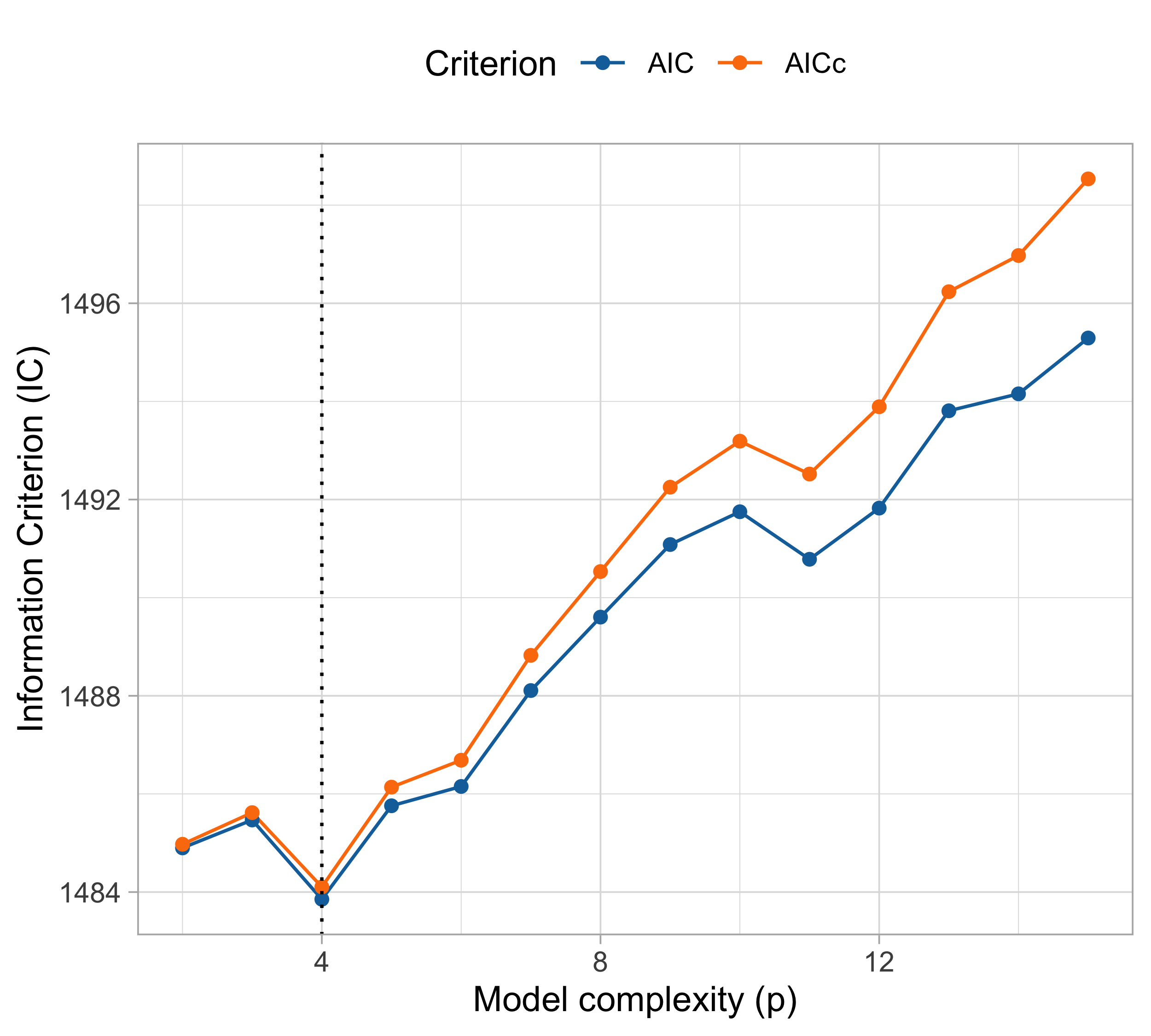
AIC, AICc, BIC

• Several other proposals followed Akaike’s original work, differing in their assumptions and the way they approximate certain quantities.

Criterion	Author	Penalty
\text{AIC}	Akaike	2p
\text{AIC}_c	Sugiura, Hurvich-Tsay	2p + \frac{2p(p+1)}{n - (p +1)}
\text{BIC}	Akaike, Schwarz	p \log{n}

• The \text{AIC}_c is an higher order correction of the \text{AIC} and the differences tend to be negligible for high values of n.

• The justification of \text{BIC} is comes from Bayesian statistics.

• Since \log{n} > 2 for any n > 7, it means that the \text{BIC} penalty is typically stronger than the one of \text{AIC} and it favors more parsimonious models.

AIC and BIC (cholesterol data)

An optimistic summary

• In the cholesterol dataset, the various indices produced different results!

  • The BIC and and the 10-fold cross-validation selected p = 2 (linear model);
  • The training/test split suggested p = 3 (quadratic model);
  • All the others (LOO-CV, \text{GCV}, \text{AIC} and \text{AIC}_c) concluded that p = 4 (cubic model).

• The good news is that all the above methods produced similar findings. For example, we are sure we should choose p \le 6.

• On the other hand, there is some uncertainty, which is quite a common situation.

• In this specific case, we may prefer p = 4, since it is based on the less-biased estimates of \text{Err}, such as the LOO-CV.

• However, this choice is debatable: another statistician may prefer the simpler linear model with p =2.

The cholesterol data: final model (p = 4)

References

• Main references
  • Chapter 3 of Azzalini, A. and Scarpa, B. (2011), Data Analysis and Data Mining, Oxford University Press.
  • Chapter 7 of Hastie, T., Tibshirani, R. and Friedman, J. (2009), The Elements of Statistical Learning, Second Edition, Springer.
• Specialized references
  • Rosset, S., and R. J. Tibshirani (2020). “From fixed-X to random-X regression: bias-variance decompositions, covariance penalties, and prediction error Estimation.” Journal of the American Statistical Association 115 (529): 138–51.
  • Bates, S., Hastie, T., and R. Tibshirani (2023). “Cross-validation: what does it estimate and how well does it do it?” Journal of the American Statistical Association, in press.