Rows: 97
Columns: 10
$ lcavol  <dbl> -0.5798185, -0.9942523, -0.5108256, -1.2039728, 0.7514161, -1.…
$ lweight <dbl> 2.769459, 3.319626, 2.691243, 3.282789, 3.432373, 3.228826, 3.…
$ age     <int> 50, 58, 74, 58, 62, 50, 64, 58, 47, 63, 65, 63, 63, 67, 57, 66…
$ lbph    <dbl> -1.3862944, -1.3862944, -1.3862944, -1.3862944, -1.3862944, -1…
$ svi     <int> 0, 0, 0, 0, 0, 0, 0, 0, 0, 0, 0, 0, 0, 0, 0, 0, 0, 0, 0, 0, 0,…
$ lcp     <dbl> -1.3862944, -1.3862944, -1.3862944, -1.3862944, -1.3862944, -1…
$ gleason <int> 6, 6, 7, 6, 6, 6, 6, 6, 6, 6, 6, 6, 7, 7, 7, 6, 7, 6, 6, 6, 6,…
$ pgg45   <int> 0, 0, 20, 0, 0, 0, 0, 0, 0, 0, 0, 0, 30, 5, 5, 0, 30, 0, 0, 0,…
$ lpsa    <dbl> -0.4307829, -0.1625189, -0.1625189, -0.1625189, 0.3715636, 0.7…
$ train <lgl> TRUE, TRUE, TRUE, TRUE, TRUE, TRUE, FALSE, TRUE, FALSE, FALSE,…Shrinkage and variable selection
Data Mining - CdL CLAMSES
Homepage

This unit will cover the following topics:
- Best subset regression
- Principal component regression
- Ridge regression
- Lasso, LARS, elastic-net
The common themes are called variable selection and shrinkage estimation.
The issue we face is the presence of a high number p of covariates that are potentially irrelevant.
This problem is quite challenging when the ratio p / n is large.
In the extreme case p > n, is there any hope of fitting a meaningful model?
A biostatistical motivation
The prostate dataset
- The
prostatecancer data investigates the relationship between the prostate-specific antigen and a number of clinical measures in men about to receive a prostatectomy.
- This dataset has been used in the original paper by Tibshirani (1996) to present the lasso. A description is given in Section 3.2.1 of HTF (2009).
We want to predict the logarithm of a prostate-specific antigen (
lpsa) as a function of:- logarithm of the cancer volume (
lcavol); - logarithm of the prostate weight (
lweight); - age each man (
age); - logarithm of the benign prostatic hyperplasia amount (
lbph); - seminal vesicle invasion (
svi), a binary variable; - logarithm of the capsular penetration (
lcp); - Gleason score (
gleason), an ordered categorical variable; - Percentage of Gleason scores 4 and 5 (
pgg45).
- logarithm of the cancer volume (
A glimpse of the prostate dataset
Summarizing, there are in total 8 variables that can be used to predict the antigen
lpsa.We centered and standardized all the covariates before the training/test split.
There are n = 67 observations in the training set and 30 in the test set.
Rows: 97
Columns: 10
$ lcavol <dbl> -1.63735563, -1.98898046, -1.57881888, -2.16691708, -0.5078744…
$ lweight <dbl> -2.00621178, -0.72200876, -2.18878403, -0.80799390, -0.4588340…
$ age <dbl> -1.86242597, -0.78789619, 1.36116337, -0.78789619, -0.25063130…
$ lbph <dbl> -1.0247058, -1.0247058, -1.0247058, -1.0247058, -1.0247058, -1…
$ svi <dbl> -0.5229409, -0.5229409, -0.5229409, -0.5229409, -0.5229409, -0…
$ lcp <dbl> -0.8631712, -0.8631712, -0.8631712, -0.8631712, -0.8631712, -0…
$ gleason <dbl> -1.0421573, -1.0421573, 0.3426271, -1.0421573, -1.0421573, -1.…
$ pgg45 <dbl> -0.8644665, -0.8644665, -0.1553481, -0.8644665, -0.8644665, -0…
$ lpsa <dbl> -0.4307829, -0.1625189, -0.1625189, -0.1625189, 0.3715636, 0.7…
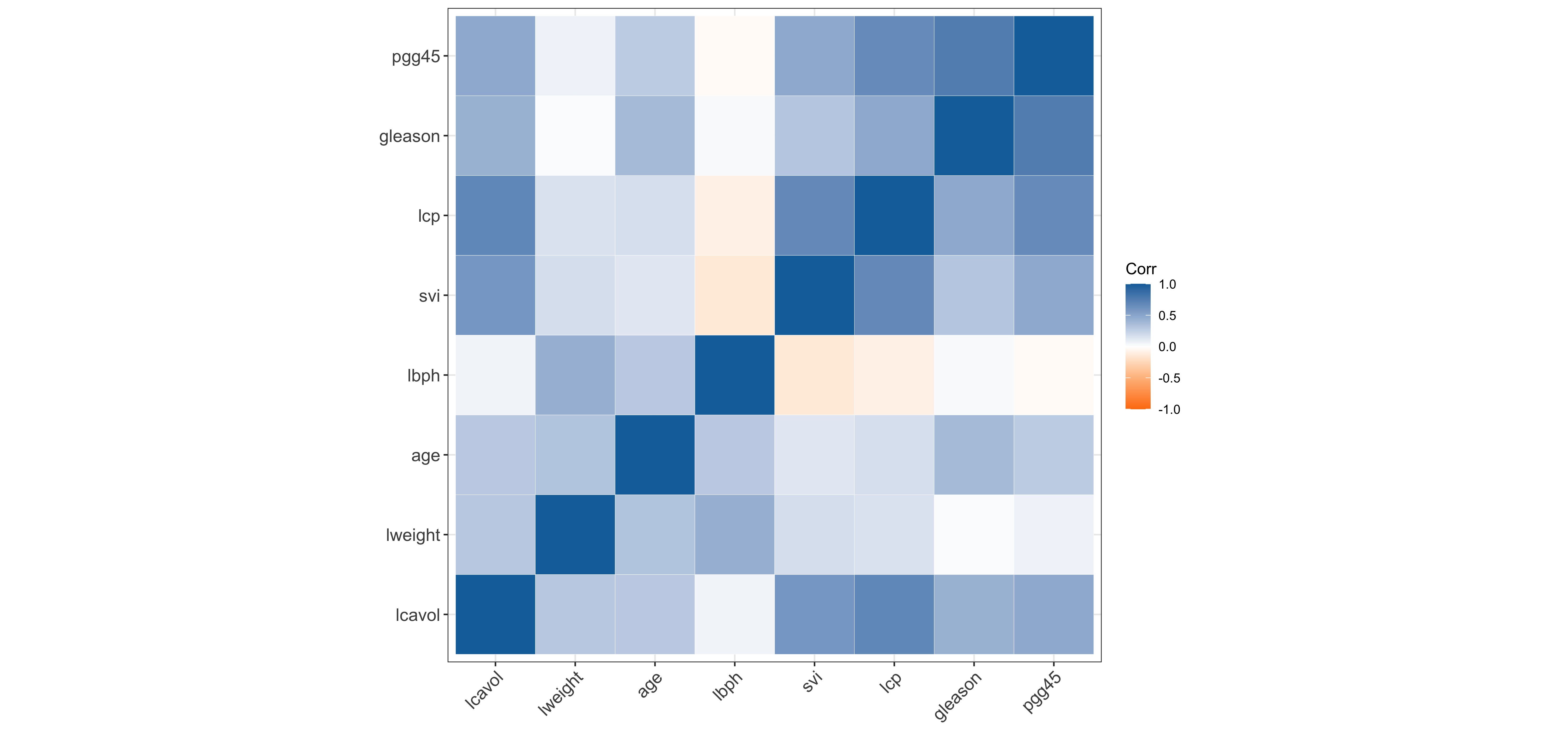
$ train <lgl> TRUE, TRUE, TRUE, TRUE, TRUE, TRUE, FALSE, TRUE, FALSE, FALSE,…Correlation matrix of prostate
The regression framework
In this unit, we will assume that the response variables Y_i (
lpsa) are obtained as Y_i = f(\bm{x}_i) + \epsilon_i, \qquad where \epsilon_i are iid random variables with \mathbb{E}(\epsilon_i) = 0 and \text{var}(\epsilon_i) = \sigma^2.Unless specifically stated, we will not assume the Gaussianity of the errors \epsilon_i nor make any specific assumption about f(\bm{x}), which could be non-linear.
In practice, we approximate the true f(\bm{x}) using a linear model, e.g., by considering the following function f(\bm{x}_i; \beta_0, \beta) = \beta_0+ \beta_1 x_{i1} + \cdots + \beta_p x_{ip} =\beta_0 + \bm{x}_i^T\beta, in which the regression coefficients must be estimated.
In this unit, the intercept \beta_0 will often play a special role therefore we use a slightly different notation compared to Unit A.
The variable selection problem
- Including a lot of covariates in the model is not necessarily a good thing!
Indeed, some variables are likely to be irrelevant:
- they might be correlated with other covariates and therefore redundant;
- they could be uncorrelated with the response
lpsa.
If we use all the p = 8 available covariates, the estimated f(\bm{x}; \hat{\beta_0}, \hat{\beta}) might have a high variance, without an important gain in terms of bias, i.e., a large mean squared error.
We are looking for a simpler model having, hopefully, a lower mean squared error.
- These considerations are particularly relevant in cases in which p > n!
A naïve approach: (ab)using p-values
(Intercept) |
lcavol |
lweight |
age |
lbph |
svi |
lcp |
gleason |
pgg45 |
|
|---|---|---|---|---|---|---|---|---|---|
| estimate | 2.46 | 0.68 | 0.26 | -0.14 | 0.21 | 0.31 | -0.29 | -0.02 | 0.27 |
| std.error | 0.09 | 0.13 | 0.10 | 0.10 | 0.10 | 0.12 | 0.15 | 0.15 | 0.15 |
| statistic | 27.60 | 5.37 | 2.75 | -1.40 | 2.06 | 2.47 | -1.87 | -0.15 | 1.74 |
| p.value | 0.00 | 0.00 | 0.01 | 0.17 | 0.04 | 0.02 | 0.07 | 0.88 | 0.09 |
It is common practice to use the p-values to perform model selection in a stepwise fashion.
However, what if the true f(\bm{x}) were not linear?
In many data mining problems, a linear model is simply an approximation of the unknown f(\bm{x}) and hypothesis testing procedures are ill-posed.
Even if the true function were linear, using p-values would not be a good idea, at least if done without appropriate multiplicity corrections.
The above p-values are meant to be used in the context of a single hypothesis testing problem, not to make iterative choices.
The predictive culture
“All models are approximations. Essentially, all models are wrong, but some are useful.”
George E. P. Box
If the focus is on prediction, we do not necessarily care about selecting the “true” set of parameters.
In many data mining problems, the focus is on minimizing the prediction errors.
Hence, often we may accept some bias (i.e., we use a “wrong” but useful model), if this leads to a reduction in variance.
Overview of this unit
In this unit, we will discuss two “discrete” methods:
- Best subset selection and its greedy approximations: forward / backward regression;
- Principal components regression (PCR).
Best subset selection perform variable selection, whereas principal components regression reduces the variance of the coefficients.
These “discrete” methods can be seen as the naïve counterpart of more advanced and continuous ideas that are presented in the second part of the Unit.
| Shrinkage | Variable selection | |
|---|---|---|
| Discrete | Principal component regression | Best subset selection, stepwise |
| Continuous | Ridge regression | Relaxed Lasso |
- Finally, the lasso and the elastic-net perform both shrinkage and variable selection.
Overview of the final results
| Least squares | Best subset | PCR | Ridge | Lasso | |
|---|---|---|---|---|---|
(Intercept) |
2.465 | 2.477 | 2.455 | 2.467 | 2.468 |
lcavol |
0.680 | 0.740 | 0.287 | 0.588 | 0.532 |
lweight |
0.263 | 0.316 | 0.339 | 0.258 | 0.169 |
age |
-0.141 | . | 0.056 | -0.113 | . |
lbph |
0.210 | . | 0.102 | 0.201 | . |
svi |
0.305 | . | 0.261 | 0.283 | 0.092 |
lcp |
-0.288 | . | 0.219 | -0.172 | . |
gleason |
-0.021 | . | -0.016 | 0.010 | . |
pgg45 |
0.267 | . | 0.062 | 0.204 | . |
Best subset selection
Best subset selection
Let us return to our variable selection problem.
In principle, we could perform an exhaustive search considering all the 2^p possible models and then selecting the one having the best out-of-sample predictive performance.
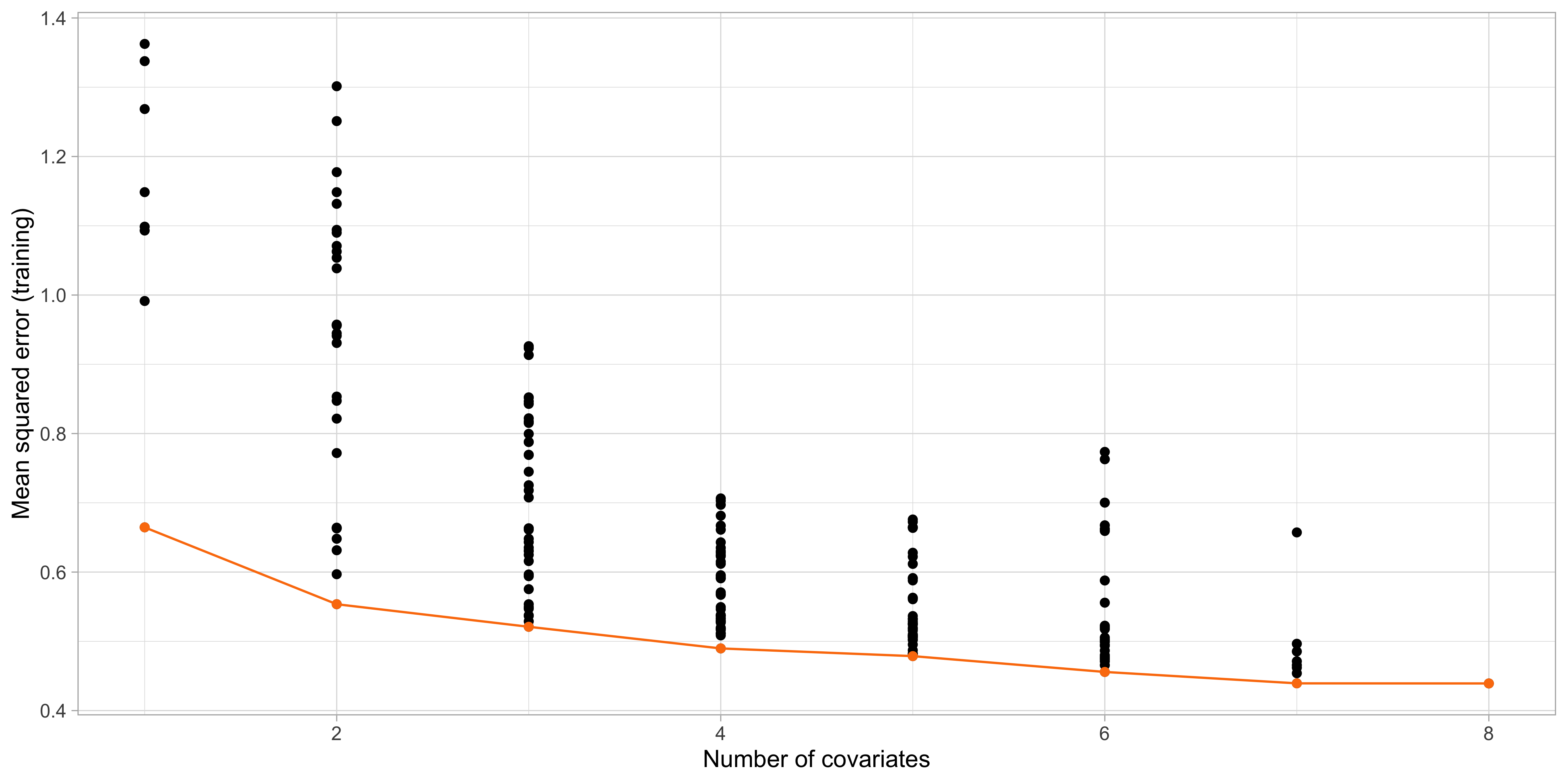
- A model with more variables has lower training error, namely \text{MSE}_{k + 1, \text{train}} \le \text{MSE}_{k, \text{train}} by construction. Hence, the optimal subset size k must be chosen e.g., via cross-validation.
Step 1. and 2. of best subset selection
The “best” models \mathcal{M}_1,\dots, \mathcal{M}_p
- The output of the best subset selection, on the training set is:
         lcavol lweight age lbph svi lcp gleason pgg45
1  ( 1 ) "*"    " "     " " " "  " " " " " "     " "
2  ( 1 ) "*"    "*"     " " " "  " " " " " "     " "
3  ( 1 ) "*"    "*"     " " " "  "*" " " " "     " "
4  ( 1 ) "*"    "*"     " " "*"  "*" " " " "     " "
5  ( 1 ) "*"    "*"     " " "*"  "*" " " " "     "*"
6  ( 1 ) "*"    "*"     " " "*"  "*" "*" " "     "*"
7  ( 1 ) "*"    "*"     "*" "*"  "*" "*" " "     "*"
8  ( 1 ) "*"    "*"     "*" "*"  "*" "*" "*"     "*"
The above table means that the best model with k = 1 uses the variable
lcavol, whereas when k = 2 the selected variables arelcavolandlweight, and so on.Note that, in general, these models are not necessarily nested, i.e. a variable selected at step k is not necessarily included at step k +1. Here they are, but it is a coincidence.
- What is the optimal subset size k in terms of out-of-sample mean squared error?
The wrong way of doing cross-validation
Consider a regression problem with a large number of predictors (relative to n) such as the
prostatedataset.A typical strategy for analysis might be as follows:
Screen the predictors: find a subset of “good” predictors that show a reasonably strong correlation with the response;
Using this subset of predictors (e.g.,
lcavol,lweightandsvi), build a regression model;Use cross-validation to estimate the prediction error of the model of the step 2.
Is this a correct application of cross-validation?
If your reaction was “this is absolutely wrong!”, it means you correctly understood the principles of cross-validation.
If you thought this was an ok-ish idea, you may want to read Section 7.10.2 of HTF (2009), called “the wrong way of doing cross-validation”.
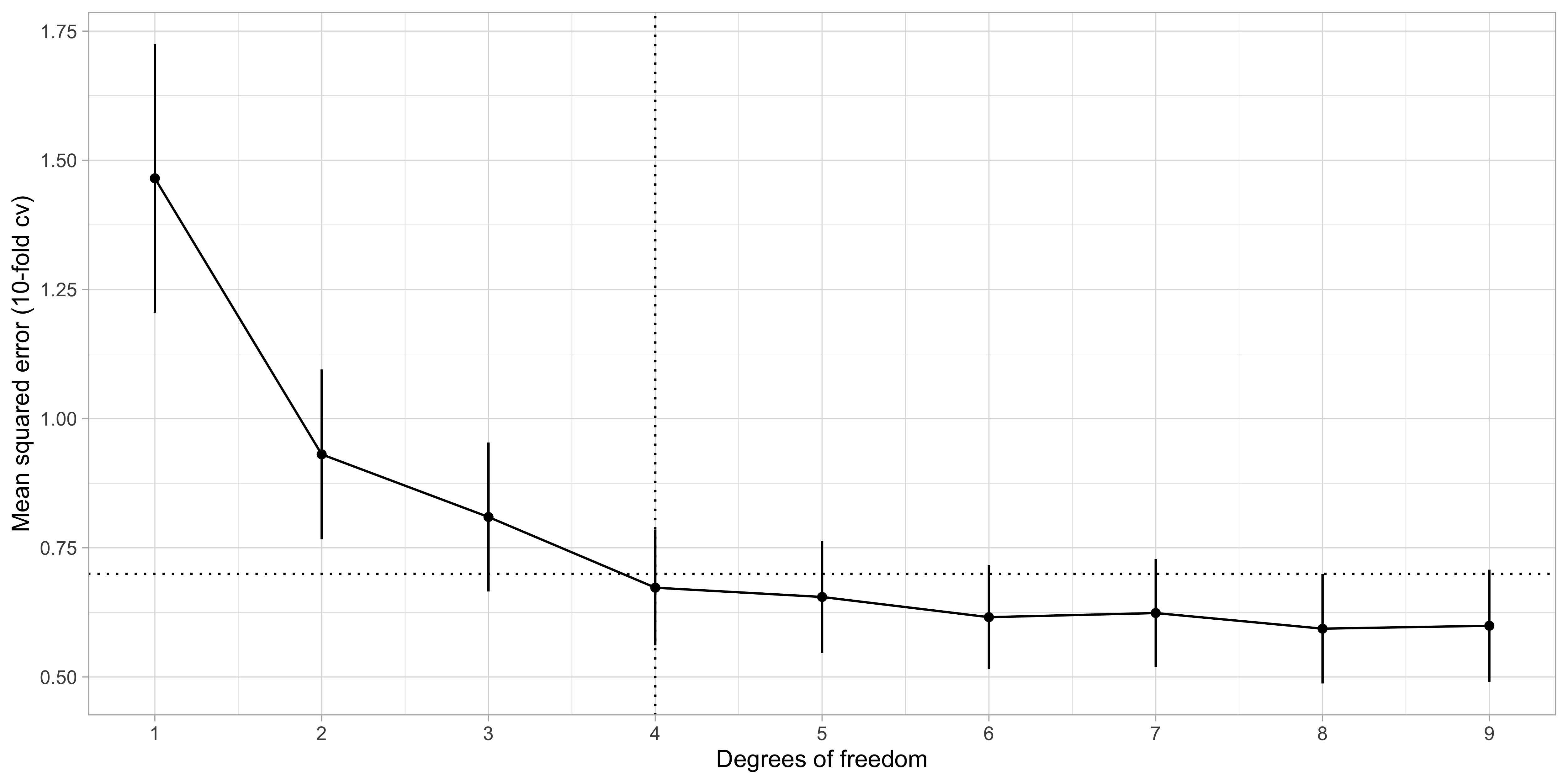
Step 3. of best subset selection via cross-validation
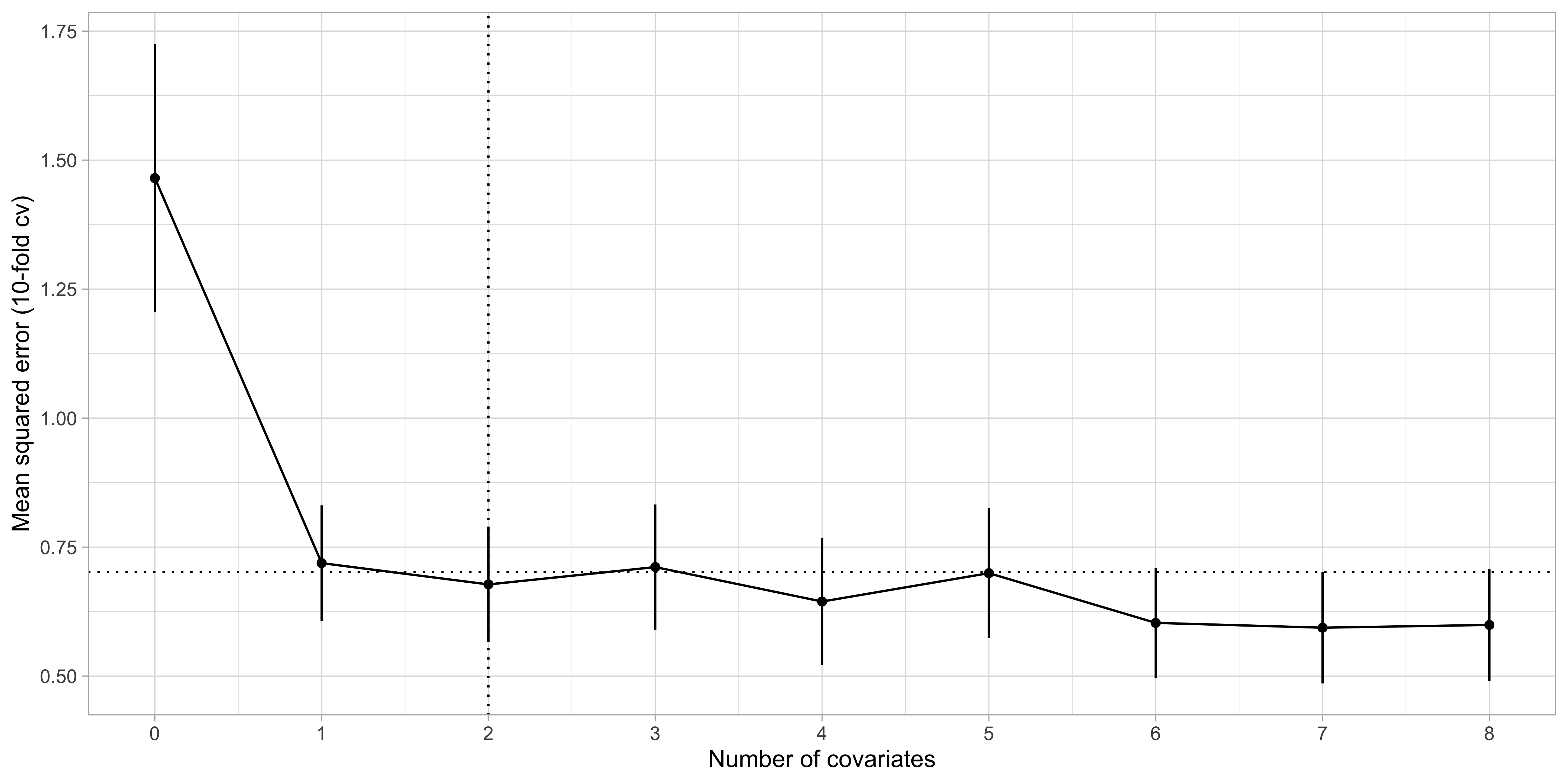
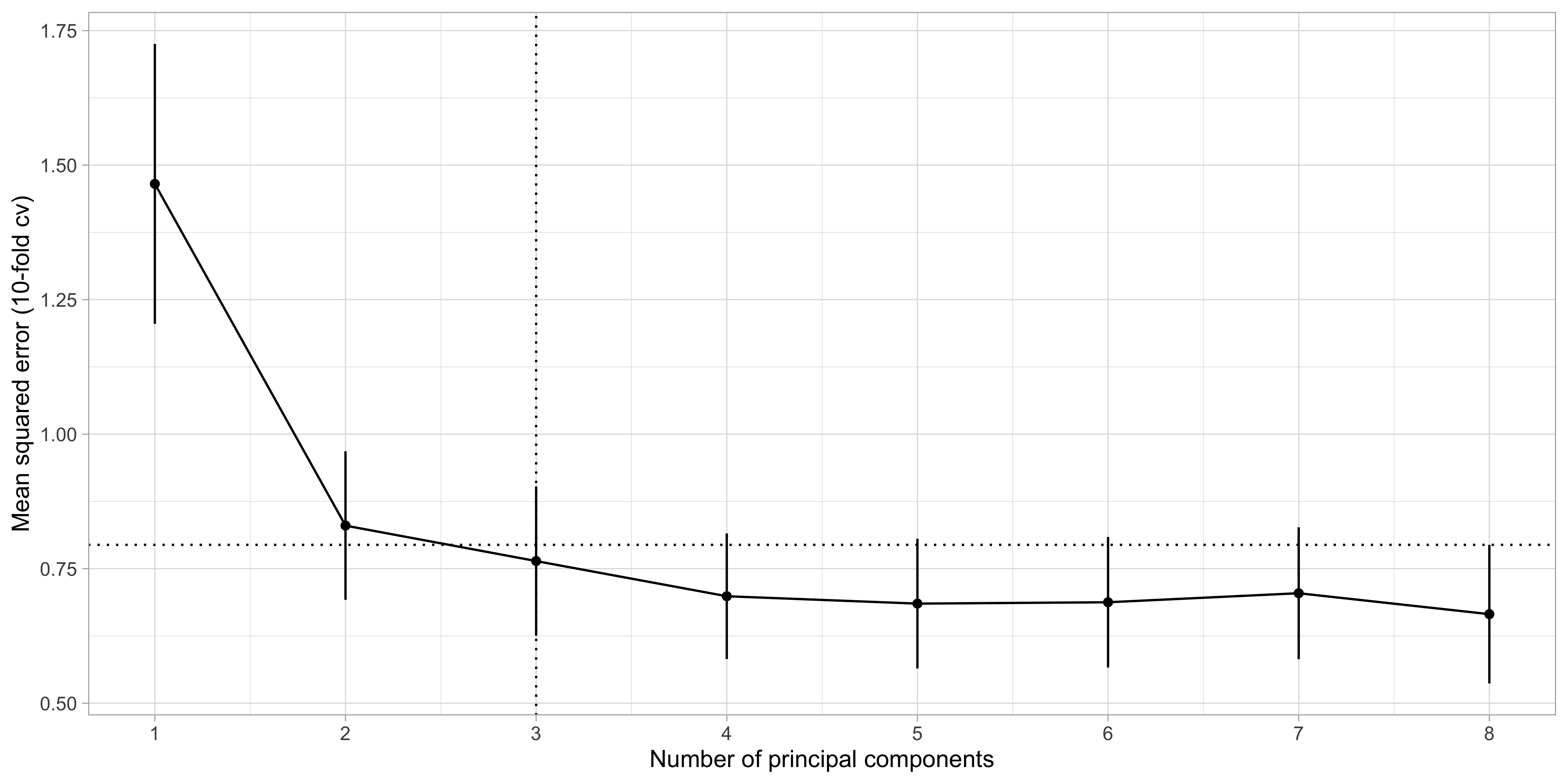
- By applying the “1 standard error rule”, we select k = 2, i.e.
lcavolandlweight.
Forward regression
- Forward regression is greedy approximation of best subset selection that produces a sequence of nested models. It is computationally feasible and can be applied when p > n.
- It can be shown that the identification of the optimal new predictor can be efficiently computed e.g. using the QR decomposition.
Backward regression
- When p < n, an alternative greedy approach is backward regression, which also produces a sequence of nested models.
- It can be shown that the dropped predictor is the one with the lowest absolute Z-score or, equivalently, the highest p-value.
Forward, backward and best subset
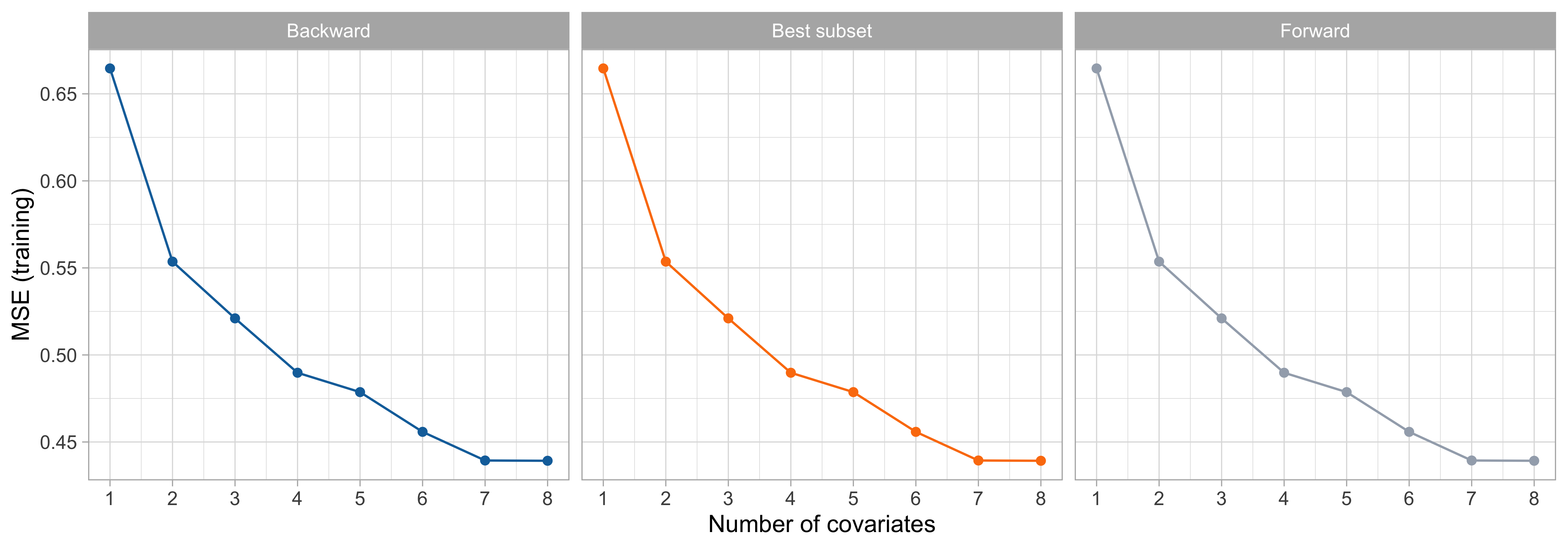
- In the
prostatedataset, forward, backward and best subset selection all gave precisely the same path of solutions on the full training set.
Pros and cons of subset selection strategies
Principal components regression
Data compression
![]()
At this point, we established that many covariates = many problems.
Instead of selecting the “best” variables, let us consider a different perspective.
We consider a compressed version of the covariates that has smaller dimension k but retains most information.
Intuitively, we want to reduce the variance by finding a good compression without sacrificing too much bias.
The main statistical tool, unsurprisingly, will be the celebrated principal components analysis (PCA).
We will compress the covariate information \bm{X} using a smaller set of variables \bm{Z}, i.e. the principal components.
The intercept term
In principal component regression and other related methods (ridge, lasso, and elastic-net), we do not wish to compress the intercept term \beta_0. We would like to “remove it”.
Let us consider a reparametrization of the linear model, in which \alpha = \beta_0 + \bar{\bm{x}}^T\beta. This is equivalent to a linear model with centered predictors: \begin{aligned} f(\bm{x}_i; \alpha, \beta) & = \beta_0 + \bm{x}_i^T\beta = \alpha - \bar{\bm{x}}^T\beta + \bm{x}_i^T\beta = \alpha + (\bm{x}_i -\bar{\bm{x}})^T\beta. \\ \end{aligned}
The estimates for (\alpha, \beta) can be now computed separately and in two steps.
The estimate of the intercept with centered predictors is \hat{\alpha} = \bar{y}. In fact: \hat{\alpha} = \arg\min_{\alpha \in \mathbb{R}}\sum_{i=1}^n\{y_i - \alpha - (\bm{x}_i -\bar{\bm{x}})^T\beta\}^2 = \frac{1}{n}\sum_{i=1}^n\{y_i - (\bm{x}_i -\bar{\bm{x}})^T\beta\} = \frac{1}{n}\sum_{i=1}^ny_i.
Then, the estimate of \beta can be obtained considering a linear model without intercept: f(\bm{x}_i; \beta) = (\bm{x}_i -\bar{\bm{x}})^T\beta, employed to predict the centered responses y_i - \bar{y}.
Centering the predictors I
- In principal components regression, we replace original data Y_i = f(\bm{x}_i) + \epsilon_i with their centered version: x_{ij} - \bar{x}_j, \qquad y_i - \bar{y}, \qquad i=1,\dots,n; \ \ j=1,\dots,p.
- In the end, we will make predictions in the original scale, which requires a simple final adjustment. One need to compute the intercept term \hat{\beta}_0 = \bar{y} - \bar{\bm{x}}\hat{\beta}, and then compute the predictions via the formula \hat{\beta}_0 + \bm{x}_i^T\hat{\beta} = \hat{\alpha} + (\bm{x}_{i}^T - \bar{\bm{x}})\hat{\beta}.
- Remark. The centering operation is a mathematical trick that simplifies the derivation but is inconsequential from an estimation point of view.
Centering the predictors II
- Using centered predictors means that we can focus on linear models without intercept: f(\bm{x}_{i}; \beta) = x_{i1}\beta_1 + \cdots + x_{ip}\beta_p = \bm{x}_{i}^T\beta.
- Under the centering assumption, the covariance matrix of the data is simply S = \frac{1}{n} \bm{X}^T\bm{X}.
Singular value decomposition (SVD)
Let \bm{X} be a n \times p matrix. Then, its full form singular value decomposition is: \bm{X} = \bm{U} \bm{D} \bm{V}^T = \sum_{j=1}^m d_j \tilde{\bm{u}}_j \tilde{\bm{v}}_j^T, with m =\min\{n, p\} and where:
- the n \times n matrix \bm{U} = (\tilde{\bm{u}}_1, \dots, \tilde{\bm{u}}_n) is orthogonal, namely: \bm{U}^T \bm{U} = \bm{U}\bm{U}^T= I_n;
- the p \times p matrix \bm{V} = (\tilde{\bm{v}}_1,\dots,\tilde{\bm{v}}_p) is orthogonal, namely: \bm{V}^T \bm{V} = \bm{V}\bm{V}^T= I_p;
- the n \times p matrix \bm{D} has diagonal entries [\bm{D}]_{jj} = d_j, for j=1,\dots,m, and zero entries elsewhere;
The real numbers d_1 \ge d_2 \ge \cdots \ge d_m \ge 0 are called singular values.
If one or more d_j = 0, then the matrix \bm{X} is singular.
Principal component analysis I
Le us assume that p < n and that \text{rk}(\bm{X}) = p, recalling that \bm{X} is a centered matrix.
Using SVD, the matrix \bm{X}^T\bm{X} can be expressed as \bm{X}^T\bm{X} = (\bm{U} \bm{D} \bm{V}^T)^T \bm{U} \bm{D} \bm{V}^T = \bm{V} \bm{D}^T \textcolor{red}{\bm{U}^T \bm{U}} \bm{D} \bm{V}^T = \bm{V} \bm{\Delta}^2 \bm{V}^T, where \bm{\Delta}^2 = \bm{D}^T\bm{D} is a p \times p diagonal matrix with entries d_1^2,\dots,d_p^2.
This equation is at the heart of principal component analysis (PCA). Define the matrix \bm{Z} = \bm{X}\bm{V} = \bm{U}\bm{D}, whose columns \tilde{\bm{z}}_1,\dots,\tilde{\bm{z}}_p are called principal components.
The matrix \bm{Z} is orthogonal, because \bm{Z}^T\bm{Z} = \bm{D}^T\textcolor{red}{\bm{U}^T \bm{U}} \bm{D} = \bm{\Delta}^2, which is diagonal.
Moreover, by definition the entries of \bm{Z} are linear combination of the original variables: z_{ij} = x_{i1}v_{i1} + \cdots + x_{ip} v_{ip} = \bm{x}_{i}^T\tilde{\bm{v}}_j. The columns \tilde{\bm{v}}_1,\dots,\tilde{\bm{v}}_p of \bm{V} are sometimes called loadings.
Principal component analysis II
Principal components form an orthogonal basis of \bm{X}, but they are not a “random” choice, and they do not coincide with them Gram-Schmidt basis of Unit A.
Indeed, the first principal component is the linear combination having maximal variance: \tilde{\bm{v}}_1 = \arg\max_{\bm{v} \in \mathbb{R}^p} \text{var}(\bm{X}\bm{v})= \arg\max_{\bm{v} \in \mathbb{R}^p} \frac{1}{n} \bm{v}^T\bm{X}^T\bm{X} \bm{v}, \quad \text{ subject to } \quad \bm{v}^T \bm{v} = 1.
The second principal component maximizes the variance under the additional constraint of being orthogonal to the former. And so on.
The values d_1^2 \ge d_2^2 \ge \dots \ge d_p^2 > 0 are the eigenvalues of \bm{X}^T\bm{X} and correspond to the rescaled variances of each principal component, that is \text{var}(\tilde{\bm{z}}_j) = \tilde{\bm{z}}_j^T \tilde{\bm{z}}_j/n = d^2_j / n.
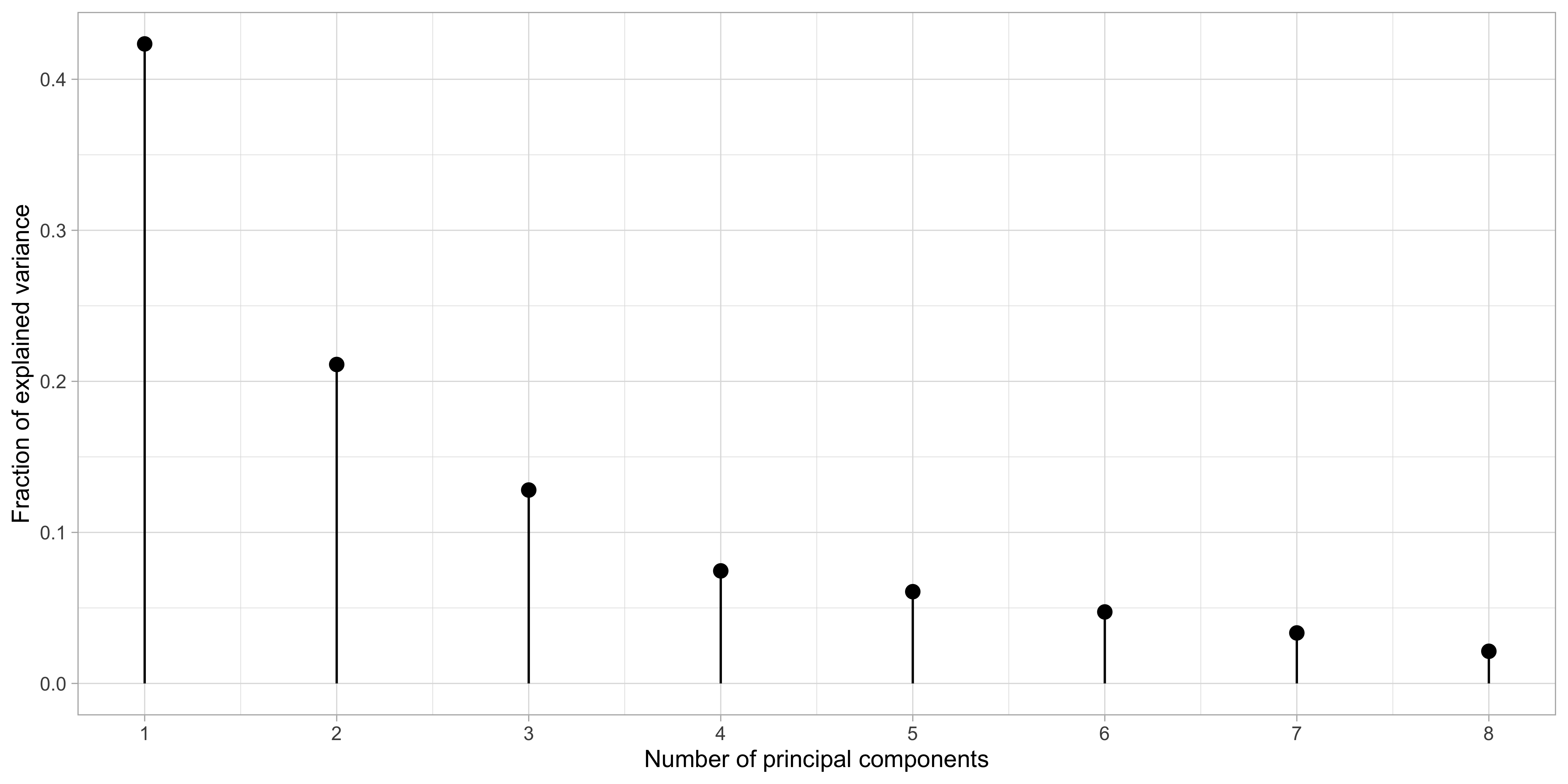
Hence, the quantity d_j^2 / \sum_{j'=1}^p d_{j'}^2 measures the amount of total variance captured by principal components.
Principal component analysis: prostate data
Principal components regression (PCR)
We use the first k \le p principal components to predict the responses y_{i} via f(\bm{z}_i; \gamma) = \gamma_1 z_{i1} + \cdots + \gamma_kz_{ik}, \qquad i=1,\dots,n,
Because of orthogonality, the least squares solution is straightforward to compute: \hat{\gamma}_j = \frac{\tilde{\bm{z}}_j^T\bm{y}}{\tilde{\bm{z}}_j^T\tilde{\bm{z}}_j} = \frac{1}{d_j^2}\tilde{\bm{z}}_j^T\bm{y}, \qquad j=1,\dots,k.
The principal components are in order of importance and effectively compressing the information contained in \bm{X} using only k \le p variables.
When k = p, we are simply rotating the original matrix \bm{X} = \bm{Z}\bm{V}, i.e. performing no compression. The predicted values coincide with OLS.
The number k is a complexity parameter which should be chosen via information criteria or cross-validation.
Selection of k: cross-validation
Shrinkage effect of principal components I
A closer look at the PCR solution reveals some interesting aspects. Recall that: \tilde{\bm{z}}_j = \bm{X}\tilde{\bm{v}}_j = d_j \tilde{\bm{u}}_j, \qquad j=1,\dots,p.
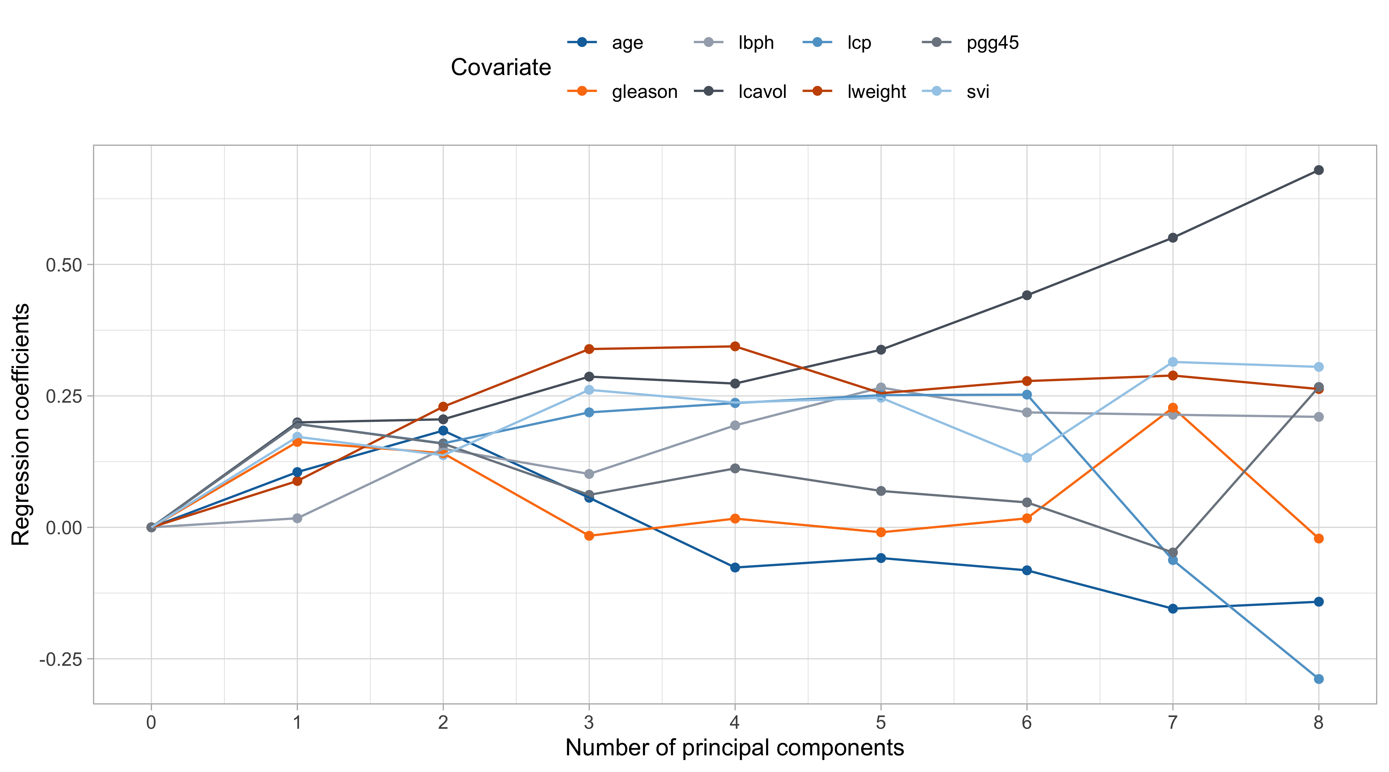
The predicted values for the centered responses \bm{y} of the PCR with k components are: \sum_{j=1}^k \tilde{\bm{z}}_j \hat{\gamma}_j = \bm{X} \sum_{j=1}^k \tilde{\bm{v}}_j \hat{\gamma}_j = \bm{X}\hat{\beta}_\text{pcr}, \qquad \text{ where } \qquad \hat{\beta}_\text{pcr} = \sum_{j=1}^k \tilde{\bm{v}}_j \hat{\gamma}_j.
This representation highlights two important aspects:
- It is possible to express the PCR solution in the original scale, for better interpretability;
- The vector \hat{\beta}_\text{pcr} is a constrained solution, being a combination of k \le p coefficients, therefore reducing the complexity of the model and shrinking the coefficients.
When k = 1, then the \hat{\beta}_\text{pcr} estimate coincide with the scaled loading vector \hat{\beta}_\text{pcr} = \hat{\gamma}_1 \tilde{\bm{v}}_1;
When k = p then the \hat{\beta}_\text{pcr} coincides with ordinary least squares (see Exercises).
Shrinkage effect of principal components II
The variance of \hat{\beta}_\text{pcr}, assuming iid errors \epsilon_i in the original data, is: \text{var}(\hat{\beta}_\text{pcr}) = \sigma^2\sum_{j=1}^k \frac{1}{d_j^2} \tilde{\bm{v}}_j\tilde{\bm{v}}_j^T.
In case of multicollinearity, then the last principal components will have a small variance, i.e., a small d_j^2. Its removal, therefore, drastically reduces the variance of \hat{\beta}_\text{pcr}.
Furthermore, the predicted values for the centered data can be expressed as \bm{X}\hat{\beta}_\text{pcr} = \sum_{j=1}^k \tilde{\bm{z}}_j \hat{\gamma}_j = \sum_{j=1}^k \tilde{\bm{z}}_j \frac{\tilde{\bm{z}}_j^T\bm{y}}{\tilde{\bm{z}}_j^T\tilde{\bm{z}}_j} = \sum_{j=1}^k \textcolor{darkblue}{d_j} \tilde{\bm{u}}_j \frac{\textcolor{darkblue}{d_j}}{\textcolor{darkblue}{d_j^2}} \frac{\tilde{\bm{u}}_j^T\bm{y}}{\textcolor{red}{\tilde{\bm{u}}_j^T\tilde{\bm{u}}_j}} = \sum_{j=1}^k \tilde{\bm{u}}_j \tilde{\bm{u}}_j^T \bm{y}.
The columns of \bm{U}, namely the vectors \tilde{\bm{u}}_j are the normalized principal components.
Hence, we are shrinking the predictions towards the main principal directions.
Shrinkage effect of principal components III
Pros and cons of PCR
Ridge regression
Shrinkage methods

Shrinkage methods are popular tools for handling the issue of multiple variables.
Shrinkage regularizes the estimates, constraining the size of the regression coefficients.
This leads to biased estimator with, hopefully, lower variance.
As a byproduct, the induced regularization procedure enables estimation even when p > n.
The first method that has been proposed is called ridge regression. The lasso and the elastic-net are other examples.
The ridge regularization method
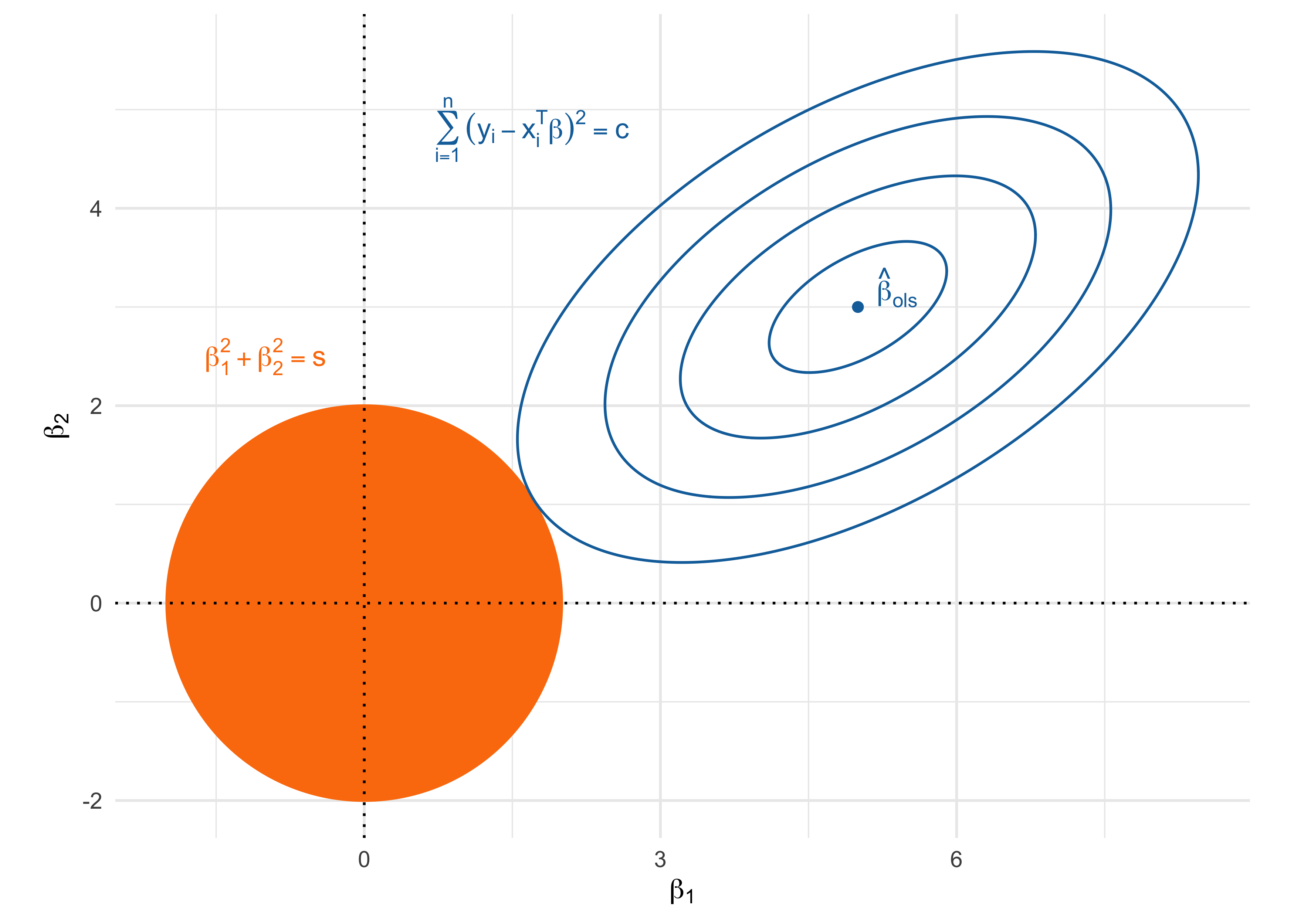
- The ridge estimator is the most common shrinkage method and is the minimizer of \sum_{i=1}^n(y_i - \beta_0 - \bm{x}_i^T\beta)^2 \qquad \text{subject to} \qquad \sum_{j=1}^p \beta_j^2 \le s.
When the complexity parameter s is small, the coefficients are explicitly shrunk, i.e. biased, towards zero.
On the other hand, if s is large enough, then the ridge estimator coincides with ordinary least squares.
- In ridge regression, the variability of the estimator is explicitly bounded, although this comes with some bias. The parameter s controls the bias-variance trade-off.
- The intercept term \beta_0 is not penalized because there are no strong reasons to believe that the mean of y_i equals zero. However, as before, we want to “remove the intercept”.
Centering and scaling the predictors I
- The ridge solutions are not equivariant under scalings of the input, so one normally standardizes the input to have unit variance if they are not on the same scale.
- Moreover, as for PCR, we can estimate the intercept using a two-step procedure:
- The reparametrization \alpha = \beta_0 + \bar{\bm{x}}^T\beta is equivalent to centering the predictors;
- The estimate for the centered intercept is \hat{\alpha} = \bar{y};
- The ridge estimate can be obtained by considering a model without intercept, using centered responses and predictors.
- Hence, in ridge regression, we replace original data Y_i = f(\bm{x}_i) + \epsilon_i with their standardized version: \frac{x_{ij} - \bar{x}_j}{s_j}, \qquad y_i - \bar{y}, \qquad i=1,\dots,n; \ \ j=1,\dots,p. where s_j^2 = n^{-1}\sum_{i=1}^n (x_{ij} - \bar{x}_j)^2 is the sample variance.
Centering and scaling the predictors II
- It is easy to show (see Exercises) that the coefficients expressed in the original scale are \hat{\beta}_0 = \bar{y} - \bar{\bm{x}}\hat{\beta}_\text{scaled-ridge}, \qquad \hat{\beta}_\text{scaled-ridge} = \text{diag}(1 / s_1,\dots, 1/s_p) \hat{\beta}_\text{ridge}. Thus, the predictions on the original scale are \hat{\beta}_0 + \bm{x}_i^T\hat{\beta}_\text{scaled-ridge} = \bar{y} + \bm{x}_{i}^T\hat{\beta}_\text{ridge}.
- We will say that the ridge estimator \hat{\beta}_\text{ridge} is the minimizer of following system \sum_{i=1}^n(y_i - \bm{x}_{i}^T\beta)^2 \qquad \text{subject to} \qquad \sum_{j=1}^p \beta_j^2 \le s.
Lagrange multipliers and ridge solution 📖
- The ridge regression problem can be equivalently expressed in its Lagrangian form, which greatly facilitates computations. The ridge estimator \hat{\beta}_\text{ridge} is the minimizer of \sum_{i=1}^n(y_{i} - \bm{x}_{i}^T\beta)^2 + \lambda \sum_{j=1}^p\beta_j^2 = \underbrace{||\bm{y} - \bm{X}\beta||^2}_{\text{least squares}} + \underbrace{\lambda ||\beta||^2}_{\text{\textcolor{red}{ridge penalty}}}, where \lambda > 0 is a complexity parameter controlling the penalty. It holds that s = ||\hat{\beta}_\text{ridge} ||^2.
- When \lambda = 0 then \hat{\beta}_\text{ridge} = \hat{\beta}_\text{ols} whereas when \lambda \rightarrow \infty we get \hat{\beta}_\text{ridge} = 0.
The geometry of the ridge solution
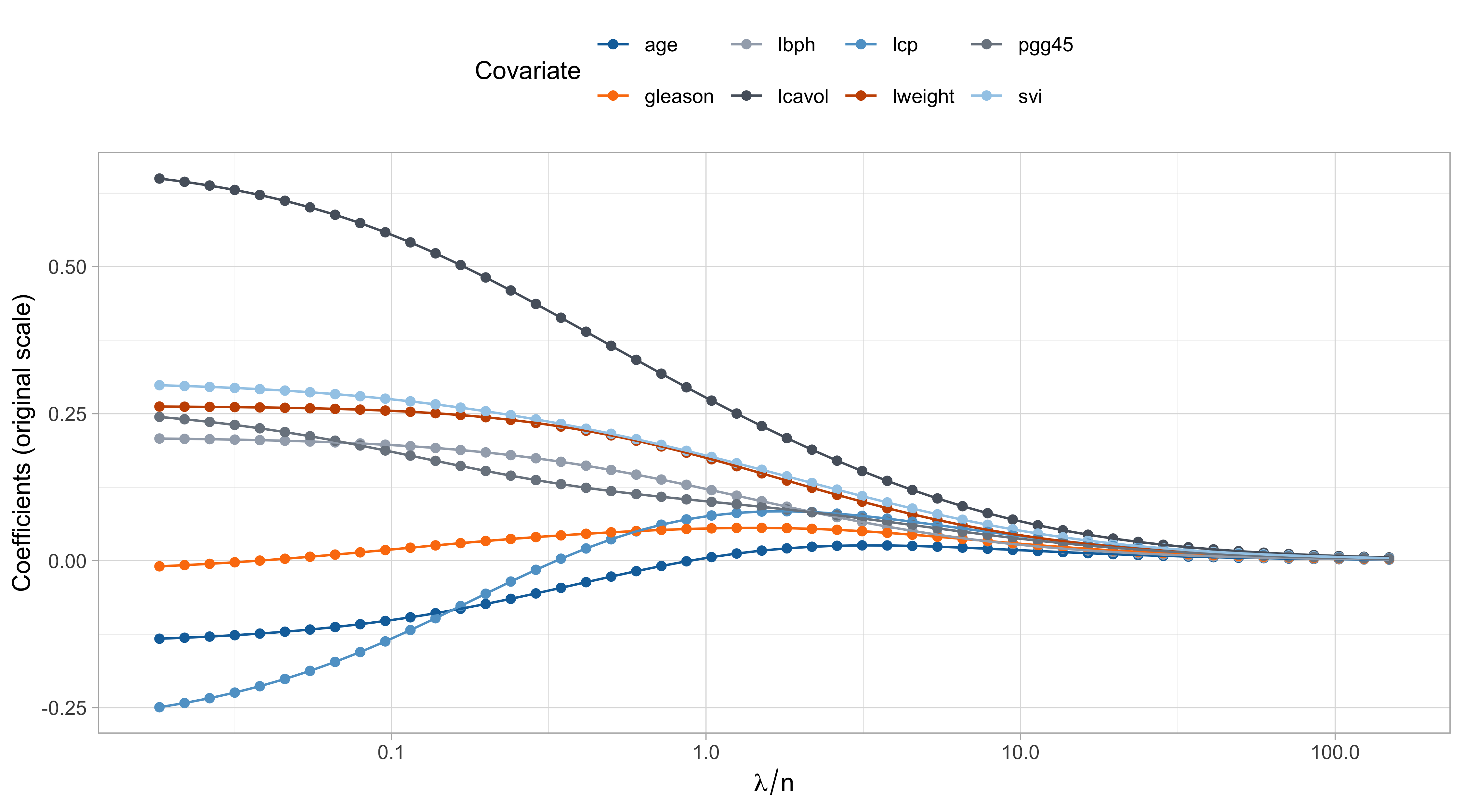
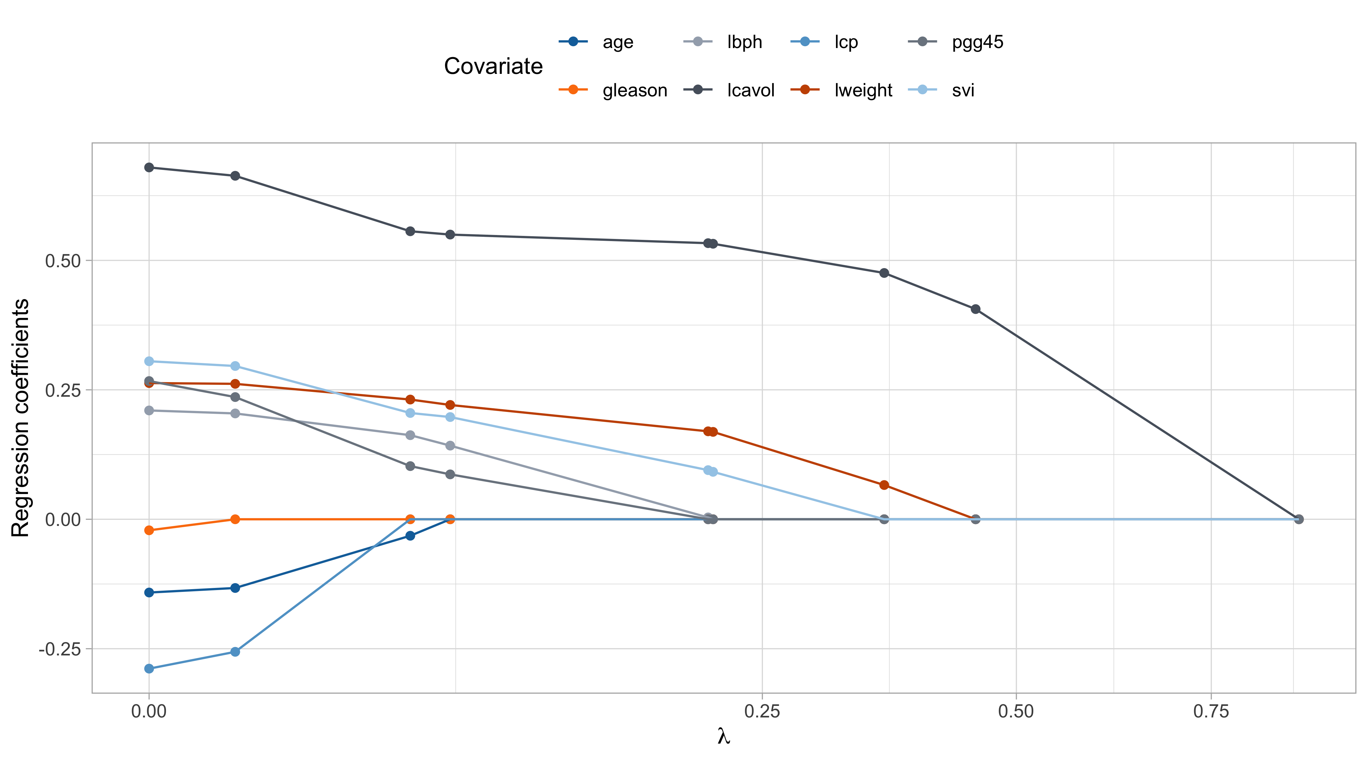
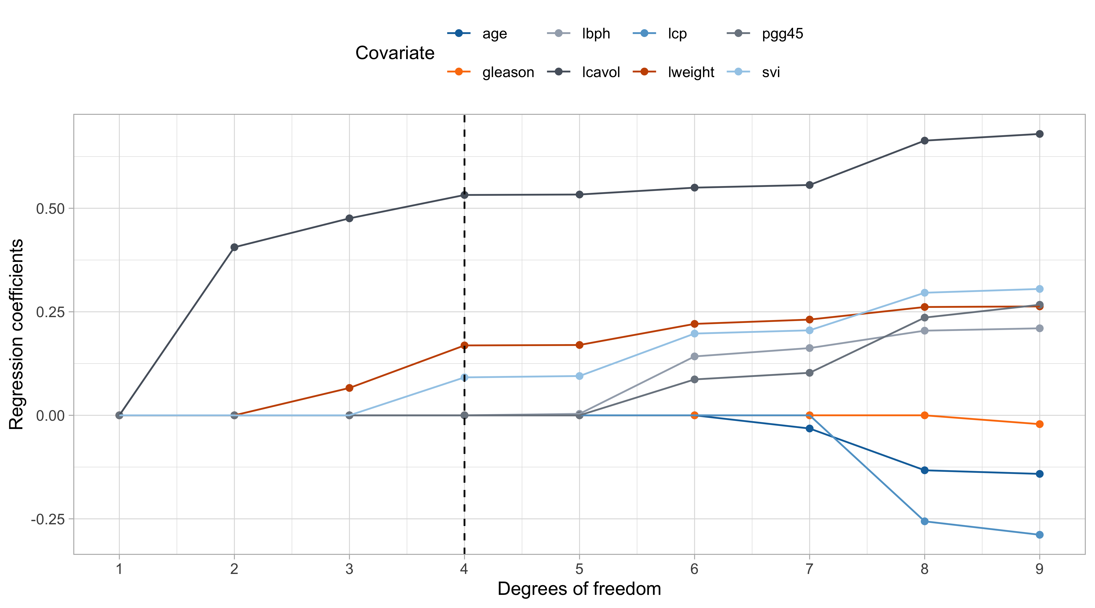
The ridge path
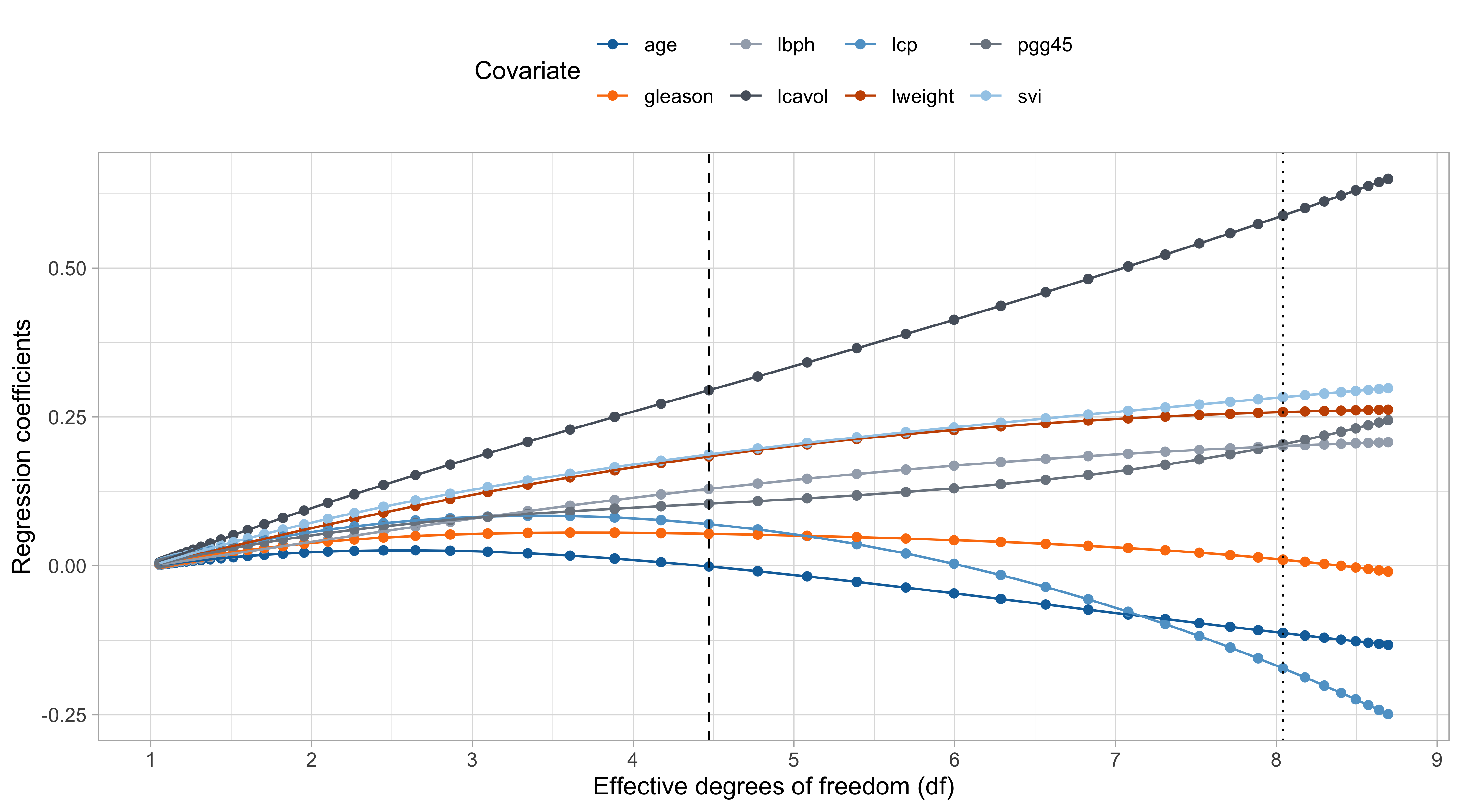
Comments on the ridge path
The values of \lambda are in somewhat arbitrary scale. The ridge penalty has a concrete effect starting from \lambda / n > 0.1 or so.
The variable
lcavolis arguably the most important, followed bylweightandsvi, which are those receiving less shrinkage compared to the others.
The coefficient of
age,gleason, andlcp, is negative at the beginning and then becomes positive for large values of \lambda.This indicate that their negative value in \hat{\beta}_\text{ols} was probably a consequence of their correlation with other variables.
- There is an interesting similarity between this plot and the one of principal component regression… is it a coincidence?
Shrinkage effect of ridge regression I
- Considering, once again, the singular value decomposition, we get: \begin{aligned} \bm{X}\hat{\beta}_\text{ridge} &= \bm{X}(\bm{X}^T\bm{X} + \lambda I_p)^{-1}\bm{X}^T\bm{y} \\ & = \bm{U}\bm{D} \bm{V}^T[\bm{V}(\bm{D}^T\bm{D} + \lambda I_p)\bm{V}^T]^{-1}(\bm{U}\bm{D}\bm{V})^T\bm{y} \\ & = \bm{U}\bm{D} \textcolor{red}{\bm{V}^T\bm{V}}(\bm{D}^T\bm{D} + \lambda I_p)^{-1} \textcolor{red}{\bm{V}^T \bm{V}} \bm{D}^T \bm{U} ^T\bm{y} \\ & = \bm{U}\bm{D}(\bm{D}^T\bm{D} + \lambda I_p)^{-1}\bm{D}^T\bm{U}^T\bm{y} \\ & = \bm{H}_\text{ridge}\bm{y} = \sum_{j=1}^p \tilde{\bm{u}}_j \frac{d_j^2}{d_j^2 + \lambda}\tilde{\bm{u}}_j^T \bm{y}, \end{aligned} where \bm{H}_\text{ridge} = \bm{X}(\bm{X}^T\bm{X} + \lambda I_p)^{-1}\bm{X}^T is the so-called hat matrix of ridge regression.
This means that ridge regression shrinks the principal directions by an amount that depends on the eigenvalues d_j^2.
In other words, it smoothly reduces the impact of the redundant information.
Shrinkage effect of ridge regression II
A sharp connection with principal components regression is therefore revealed.
Compare the previous formula for \bm{X}\hat{\beta}_\text{ridge} with the one we previously obtained for \bm{X}\hat{\beta}_\text{pcr}.
- More explicitly, for ridge regression we will have that \hat{\beta}_\text{ridge} = \bm{V}\text{diag}\left(\frac{d_1}{d_1^2 + \lambda}, \dots, \frac{d_p}{d_p^2 + \lambda}\right)\bm{U}^T\bm{y}. whereas for principal components regression with k components we get \hat{\beta}_\text{pcr} = \bm{V}\text{diag}\left(\frac{1}{d_1}, \dots, \frac{1}{d_k}, 0, \dots, 0\right)\bm{U}^T\bm{y}.
- Both operate on the singular values, but where principal component regression thresholds the singular values, ridge regression shrinks them.
Bias-variance trade-off 📖
- The ridge regression add some bias to the estimates, but it reduces their variance.
- The variance of \hat{\beta}_\text{ridge}, assuming iid errors \epsilon_i in the original scale with variance \sigma^2, results: \text{var}(\hat{\beta}_\text{ridge}) = \sigma^2\sum_{j=1}^p \frac{d_j^2}{(d_j^2 + \lambda)^2} \tilde{\bm{v}}_j\tilde{\bm{v}}_j^T, whose diagonal elements are always smaller than those of \text{var}(\hat{\beta}_\text{ols}).
The above formula highlights that ridge will be very effective in presence highly correlated variables, as they will be “shrunk” away by the penalty.
What typically happens is that such a reduction in variance compensate the increase in bias, especially when p is large relative to n.
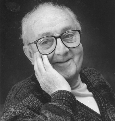
A historical perspective I
The ridge regression estimator was originally proposed by Hoerl and Kennard (1970) with a quite different motivation in mind.
In linear models, the estimate of \beta is obtained by solving the normal equations (\bm{X}^T\bm{X})\beta = \bm{X}^T\bm{y}, which could be ill-conditioned.
In other words, the condition number \kappa(\bm{X}^T\bm{X}) = \frac{d_1^2}{d_p^2}, might be very large, leading to numerical inaccuracies, since the matrix \bm{X}^T\bm{X} is numerically singular and therefore not invertible in practice.
A historical perspective II
Ridge provides a remedy for ill-conditioning, by adding a “ridge” to the diagonal of \bm{X}^T\bm{X}, obtaining the modified normal equations (\bm{X}^T\bm{X} + \lambda I_p)\beta = \bm{X}^T\bm{y}.
The condition number of the modified (\bm{X}^T\bm{X} + \lambda I_p) matrix becomes \kappa(\bm{X}^T\bm{X} + \lambda I_p) = \frac{\lambda + d_1^2}{\lambda + d_p^2}.
Notice that even if d_p = 0, i.e. the matrix \bm{X} is singular, then the condition number will be finite as long as \lambda > 0.
This technique is known as Tikhonov regularization, after the Russian mathematician Andrey Tikhonov.
A historical perspective III
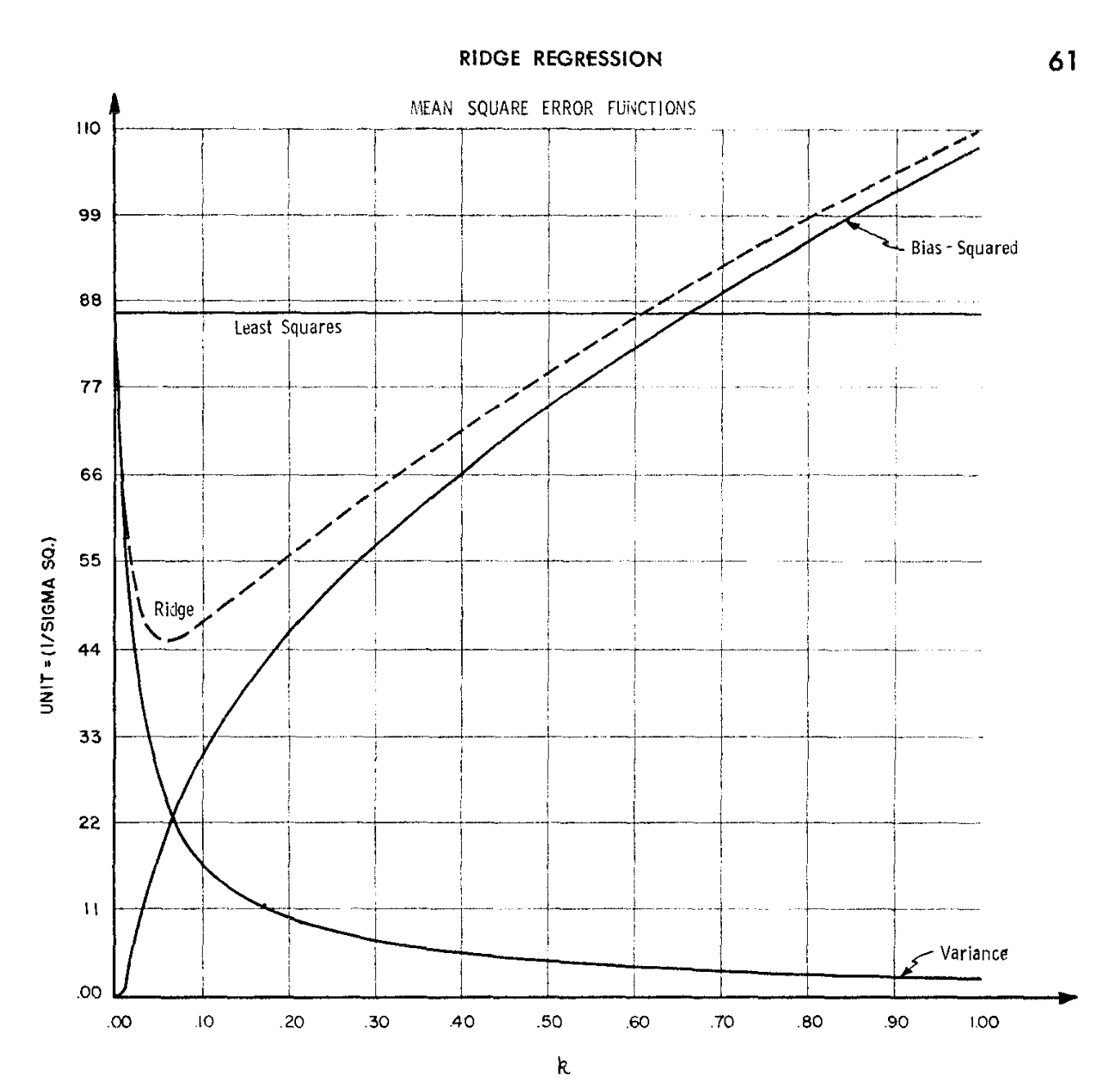
- Figure 1 of the original paper by Hoerl and Kennard (1970), displaying the bias-variance trade-off.
On the choice of \lambda
- The penalty parameter \lambda determines the amount of bias and variance of \hat{\beta}_\text{ridge} and therefore it must be carefully estimated.
Minimizing the loss ||\bm{y} - \bm{X}\hat{\beta}_\text{ridge}||^2 over \lambda is a bad idea, because it would always lead to \lambda = 0, corresponding to \hat{\beta}_\text{ridge} = \hat{\beta}_\text{ols}.
Indeed, \lambda is a complexity parameter and, like the number of covariates, should be selected using information criteria or training/test and cross-validation.
Suppose we wish to use an information criteria such as the AIC or BIC, of the form \text{IC}(p) = -2 \ell(\hat{\beta}_\text{ridge}) + \text{penalty}(\text{``degrees of freedom"}). We need a careful definition of degrees of freedom that is appropriate in this context.
The current definition of degrees of freedom, i.e., the number of non-zero coefficients, is not appropriate for ridge regression because it would be equal to p for any value of \lambda.
Effective degrees of freedom I
- Let us recall that the original data are Y_i = f(\bm{x}_i) + \epsilon_i and that the optimism for a generic estimator \hat{f}(\bm{x}) is defined as the following average of covariances \text{Opt} = \frac{2}{n}\sum_{i=1}^n\text{cov}(Y_i, \hat{f}(\bm{x}_i)), which is equal to \text{Opt}_\text{ols} = (2\sigma^2p)/ n in ordinary least squares.
Effective degrees of freedom II 📖
The effective degrees of freedom of ordinary least squares and principal component regression are \text{df}_\text{ols} = p + 1, \qquad \text{df}_\text{pcr} = k + 1, where the additional term corresponds to the intercept.
After some algebra, one finds that the effective degrees of freedom of ridge regression are \text{df}_\text{ridge} = 1 + \text{tr}(\bm{H}_\text{ridge}) = 1 + \sum_{j=1}^p \frac{d_j^2}{d_j^2 + \lambda}.
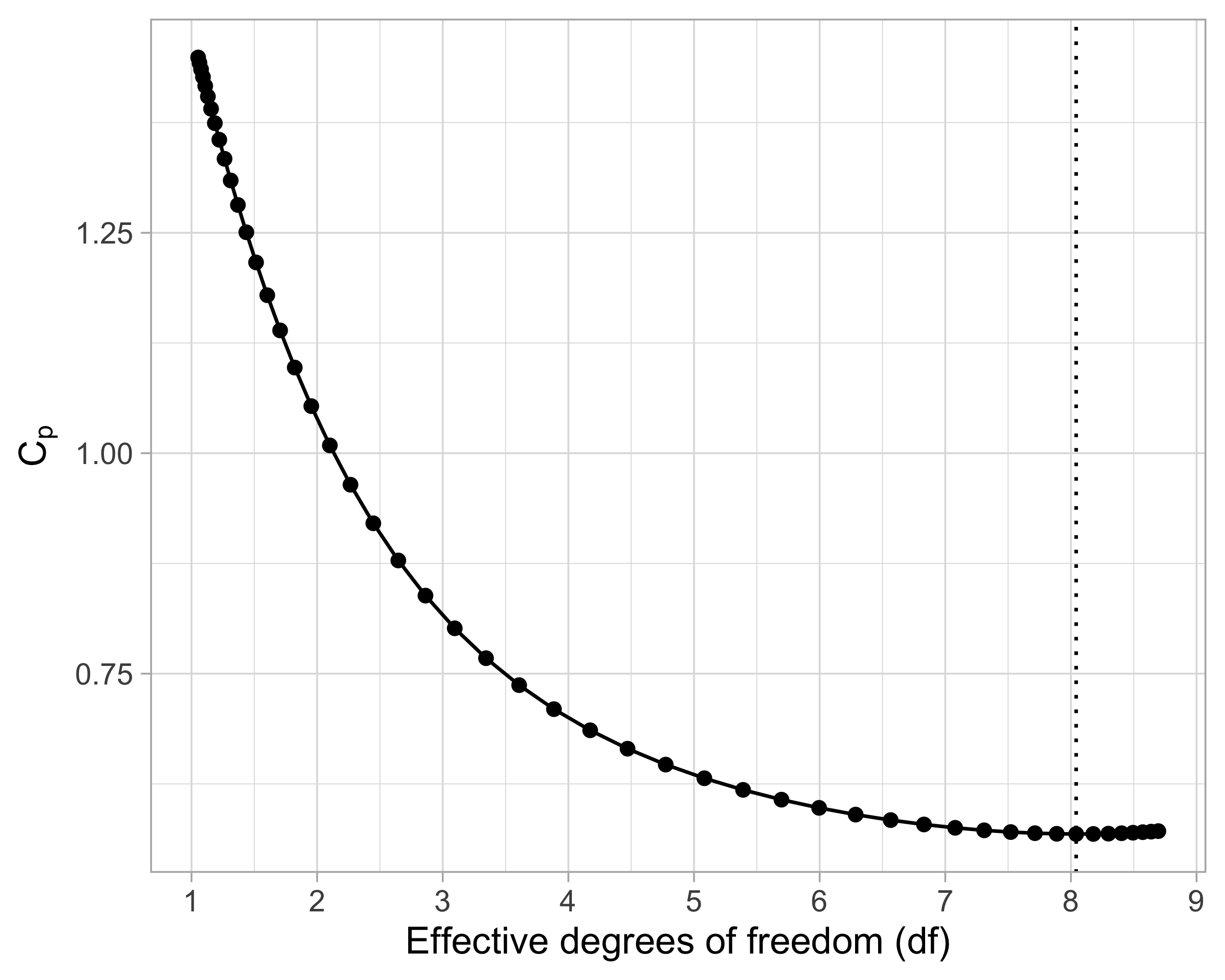
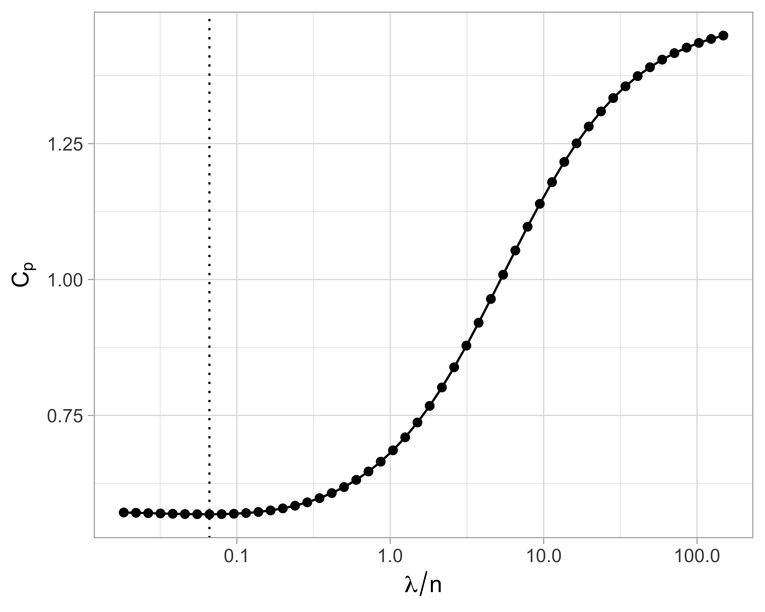
Using the above result, we can plug-in \text{df}_\text{ridge} into the formula of the C_p of Mallows: \widehat{\mathrm{ErrF}} = \frac{1}{n}\sum_{i=1}^n(y_i - \bm{x}_i^T\hat{\beta}_\text{scaled-ridge})^2 + \frac{2 \hat{\sigma}^2}{n} \text{df}_\text{ridge}. where the residual variance is estimated as \hat{\sigma}^2 = (n - \text{df}_\text{ridge})^{-1} \sum_{i=1}^n(y_i - \bm{x}_i^T\hat{\beta}_\text{scaled-ridge})^2.
Effective degrees of freedom III
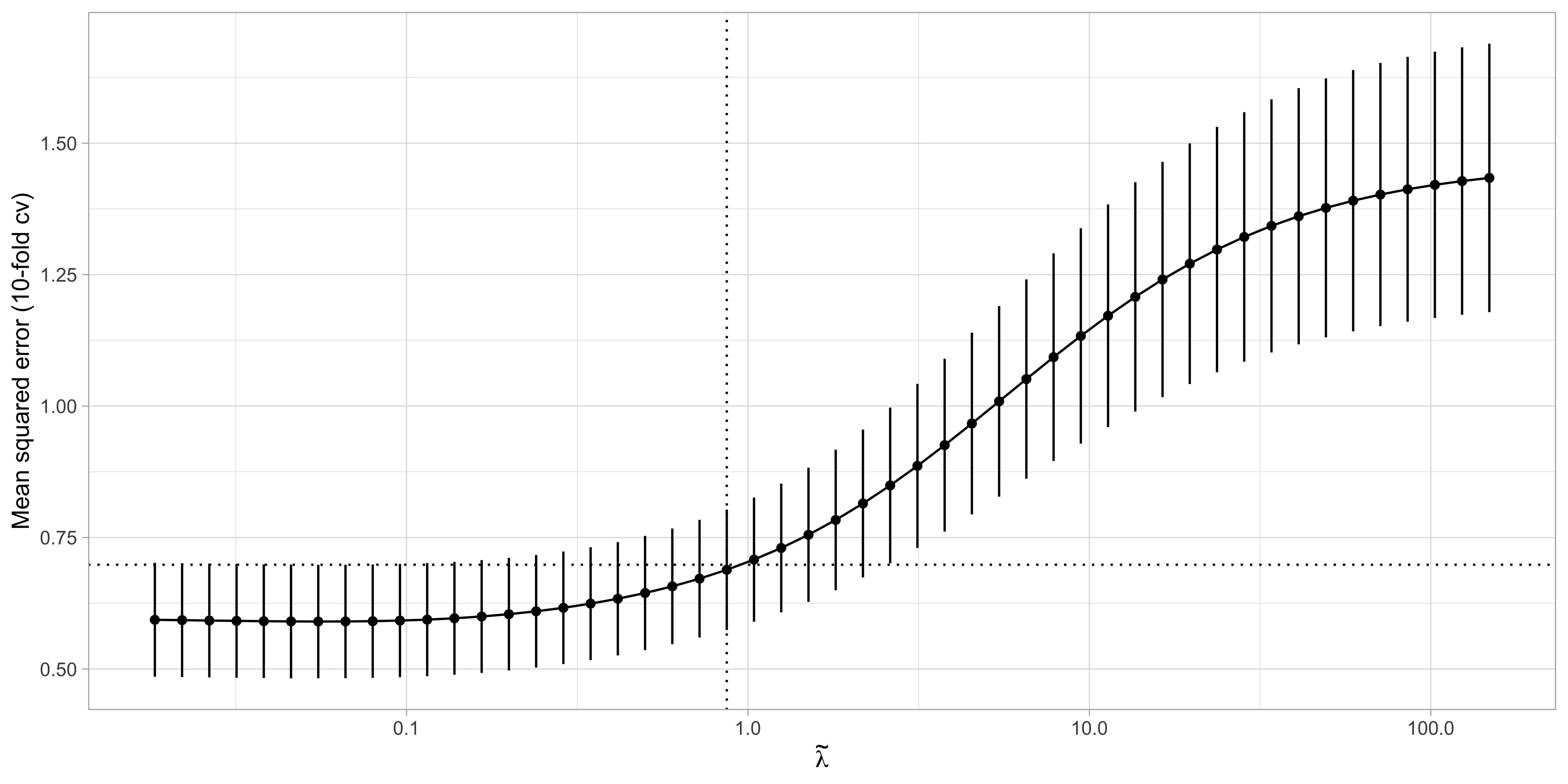
Cross-validation for ridge regression I
Training/test strategies and cross-validation are also valid tools for selecting \lambda.
Most statistical software packages use a slightly different parametrization for \lambda, as they minimize \textcolor{red}{\frac{1}{n}}\sum_{i=1}^n(y_{i} - \bm{x}_{i}^T\beta)^2 + \tilde{\lambda} \sum_{j=1}^p\beta_j^2, where the penalty parameter \tilde{\lambda} = \lambda / n.
- This parametrization does not alter the estimate of \hat{\beta}_\text{ridge} but is more amenable for cross-validation as the values of \tilde{\lambda} can be compared across datasets with different sample sizes.
Different R packages have different defaults about other aspects too.
For instance, the R package
glmnetuses \tilde{\lambda} and also standardizes the response \bm{y} and then transforms back the estimated coefficients into the original scale.
Cross-validation for ridge regression II
The ridge estimate
Further properties of ridge regression
Ridge regression has a transparent Bayesian interpretation, since the penalty can be interpreted as a Gaussian prior on \beta.
If two variables are identical copies \tilde{\bm{x}}_j = \tilde{\bm{x}}_\ell, so are the corresponding ridge coefficients \hat{\beta}_{j,\text{ridge}} = \hat{\beta}_{\ell,\text{ridge}}.
Adding p fake observations all equal to 0 to the response and then fitting ordinary least squares leads to the ridge estimator. This procedure is called data augmentation.
A computationally convenient formula for LOO cross-validation is available, which requires the model to be estimated only once, as in least squares.
In the p > n case there are specific computational strategies that can be employed; see Section 18.3.5 of Hastie, Tibshirani and Friedman (2011).
Pros and cons of ridge regression
The lasso
Looking for sparsity

- Signal sparsity is the assumption that only a small number of predictors have an effect, i.e., \beta_j = 0, \qquad \text{for most} \qquad j \in \{1,\dots,p\}.
- In this case we would like our estimator \hat{\beta} to be sparse, meaning that \hat{\beta}_j = 0 for many j \in \{1,\dots,p\}.
- Sparse estimators are desirable because:
- perform variable selection and improve the interpretability of the results;
- Speed up the computations of the predictions because fewer variables are needed.
- Best subset selection is sparse (but computationally unfeasible), the ridge estimator is not.
The least absolute selection and shrinkage operator
- The lasso was introduced in the highly influential paper of Tibshirani (1996). It is a method that performs both shrinkage and variable selection
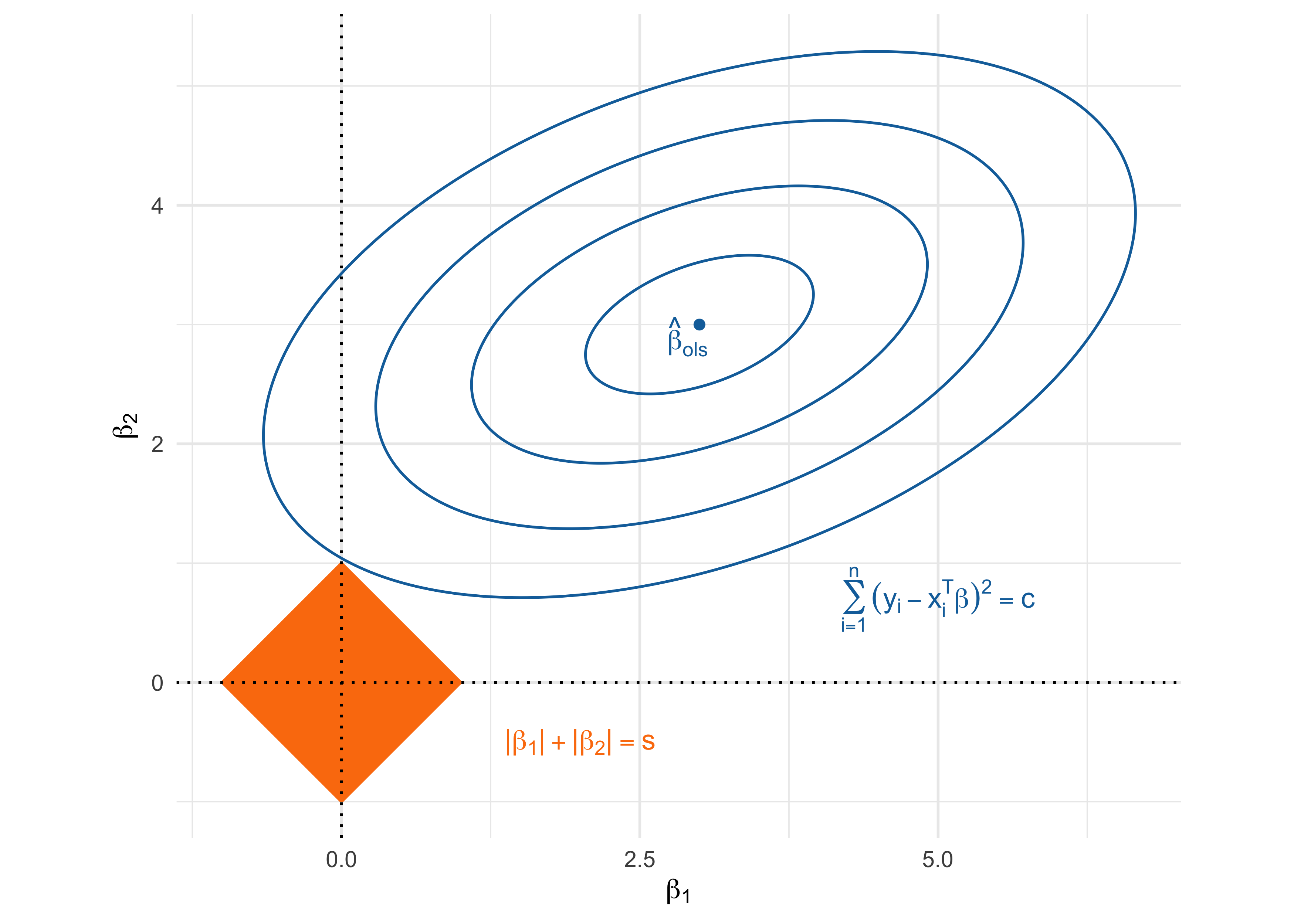
- The lasso estimator is the minimizer of the following system \sum_{i=1}^n(y_i - \beta_0- \bm{x}_i^T\beta)^2 \qquad \text{subject to} \qquad \sum_{j=1}^p |\beta_j| \le s. therefore when the complexity parameter s is small, the coefficients of \hat{\beta}_\text{lasso} are shrunk and when s is large enough \hat{\beta}_\text{lasso} = \hat{\beta}_\text{ols}, as in ridge regression.
- The lasso is deceptively similar to ridge. However, the change from a quadratic penalty to an absolute value has a crucial sparsity implication.
- The intercept term \beta_0 is not penalized, as for ridge, because we can remove it by centering the predictors.
Centering and scaling the predictors
Thus, as for ridge regression, we will center and scale predictors and response.
It is easy to show that the coefficients expressed in the original scale are \hat{\beta}_0 = \bar{y} - \bar{\bm{x}}\hat{\beta}_\text{lasso}, \qquad \hat{\beta}_\text{scaled-lasso} = \text{diag}(1 / s_1,\dots, 1/s_p) \hat{\beta}_\text{lasso}. Thus, the predictions on the original scale are \hat{\beta}_0 + \bm{x}_i^T\hat{\beta}_\text{scaled-lasso} = \bar{y} + \bm{x}_{i}^T\hat{\beta}_\text{lasso}.
- We will say that the lasso estimator \hat{\beta}_\text{lasso} is the minimizer of following system \sum_{i=1}^n(y_i - \bm{x}_{i}^T\beta)^2 \qquad \text{subject to} \qquad \sum_{j=1}^p| \beta_j| \le s.
Lagrange multipliers and lasso solution
The lasso problem can be equivalently expressed in its Lagrangian form, which is more amenable for computations.
Having removed the intercept, the lasso estimator \hat{\beta}_\text{lasso} is the minimizer of \underbrace{\textcolor{darkblue}{\frac{1}{2 n}}\sum_{i=1}^n(y_{i} - \bm{x}_i^T\beta)^2}_{\text{least squares}} + \underbrace{\lambda \sum_{j=1}^p|\beta_j|}_{\text{\textcolor{red}{lasso penalty}}} where \lambda > 0 is a complexity parameter controlling the penalty.
When \lambda = 0 the penalty term disappears and \hat{\beta}_\text{lasso} = \hat{\beta}_\text{ols}. On the other hand, there exists a finite value of \lambda_0 < \infty such that \hat{\beta}_\text{lasso} = 0.
For any intermediate value 0 < \lambda < \lambda_0 we get a combination of shrunk but positive coefficients, and a set of coefficients whose value is exactly zero.
- Unfortunately, there is no closed-form expression for the lasso solution.
The geometry of the lasso solution
Lasso with a single predictor I
To gain some understanding, let us consider the single-predictor scenario, in which \hat{\beta}_\text{lasso} = \arg\min_{\beta}\frac{1}{2n}\sum_{i=1}^n(y_{i} - x_{i}\beta)^2 + \lambda |\beta|.
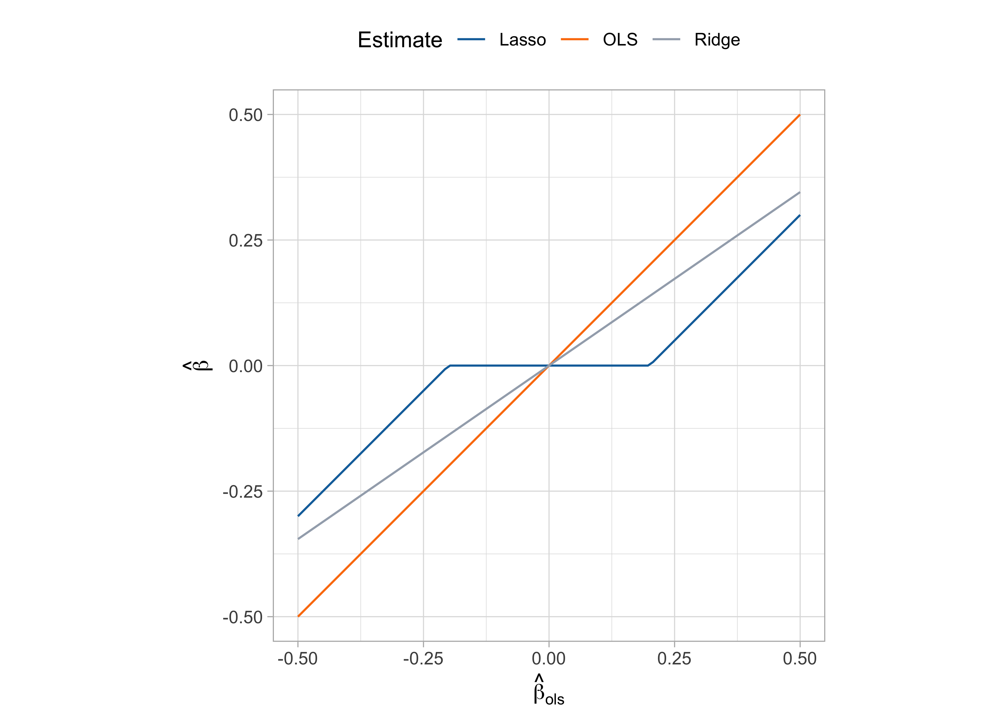
This simple problem admits an explicit expression (see Exercises), which is \hat{\beta}_\text{lasso} = \begin{cases} \text{cov}(x,y) - \lambda, \qquad &\text{if} \quad \text{cov}(x,y) > \lambda \\ 0 \qquad &\text{if} \quad |\text{cov}(x,y)| \le \lambda\\ \text{cov}(x,y) + \lambda, \qquad &\text{if} \quad \text{cov}(x,y) < -\lambda \\ \end{cases}
The above solution can be written as \hat{\beta}_\text{lasso} = \mathcal{S}_\lambda(\hat{\beta}_\text{ols}), where \mathcal{S}_\lambda(x) = \text{sign}(x)(|x| - \lambda)_+ is the soft-thresholding operator and (\cdot)_+ is the positive part of a number (
pmax(0, x)).For ridge regression (including a n^{-1} factor in the least squares penalty; see here) we get: \hat{\beta}_\text{ridge} = \frac{1}{\lambda + 1}\text{cov}(x,y) =\frac{1}{\lambda + 1}\hat{\beta}_\text{ols} = \frac{1}{\lambda + 1}\frac{1}{n}\sum_{i=1}^n x_{i}y_{i}.
Lasso with a single predictor II
Soft-thresholding and lasso solution
- The single predictor special case provides further intuition of why the lasso perform variable selection and shrinkage.
Ridge regression induces shrinkage in a multiplicative fashion, and the regression coefficients reach zero as \lambda \rightarrow \infty.
Conversely, the lasso shrinks the ordinary least squares in an additive manner, truncating them at zero after a certain threshold.
- Even though we do not have a closed-form expression for the lasso solution \hat{\beta}_\text{lasso} when the covariates p > 1, the main intuition is preserved: lasso induces sparsity!
The lasso path
Least angle regression I
- Least angle regression (LAR) is a “democratic” version of forward stepwise regression.
Forward stepwise builds a model sequentially, adding one variable at a time. At each step, the best variable is included in the active set and then the least square fit is updated.
LAR uses a similar strategy, but any new variable contributes to the predictions only “as much” as it deserves.
Least angle regression: remarks 📖
- The coefficients in LAR change in a piecewise fashion, with knots in \lambda_k. The LAR path coincides almost always with the lasso. Otherwise, a simple modification is required:
☠️ - Lasso and LAR relationship
- What follows is heuristic intuition for why LAR and lasso are so similar. By construction, at any stage of the LAR algorithm, we have that: \text{cov}(\tilde{\bm{x}}_j, \bm{r}(\lambda)) = \frac{1}{n}\sum_{i=1}^nx_{ij}\{y_i - \bm{x}_i^T\beta(\lambda)\} = \lambda s_j, \qquad j \in \mathcal{A}, where s_j \in \{-1, 1\} indicates the sign of the covariance.
- On the other hand, let \mathcal{A}_\text{lasso} be the active set of the lasso. For these variables, the penalized lasso loss is differentiable, obtaining: \text{cov}(\tilde{\bm{x}}_j, \bm{r}(\lambda)) = \frac{1}{n}\sum_{i=1}^nx_{ij}\{y_i - \bm{x}_i^T\beta(\lambda)\} = \lambda \text{sign}(\beta_j), \qquad j \in \mathcal{A}_\text{lasso}, which coincide with the LAR solution if s_j = \text{sign}(\beta_j), which is almost always the case.
Uniqueness of the lasso solution
- The lasso can be computed even when p > n. In these cases, will it be unique?
Non-uniqueness may occur in the presence of discrete-valued data. It is of practical concern only whenever p > n and if we are interested in interpreting the coefficients.
Much more general sufficient conditions for the uniqueness of \hat{\beta}_\text{lasso} are known, but they are quite technical and complex to check in practice.
The degrees of freedom of the lasso
- In ridge regression, the effective degrees of freedom have a simple formula.
- Miraculously, for the lasso with a fixed penalty parameter \lambda, the number of nonzero coefficients |\mathcal{A}_\text{lasso}(\lambda)| is an unbiased estimate of the degrees of freedom.
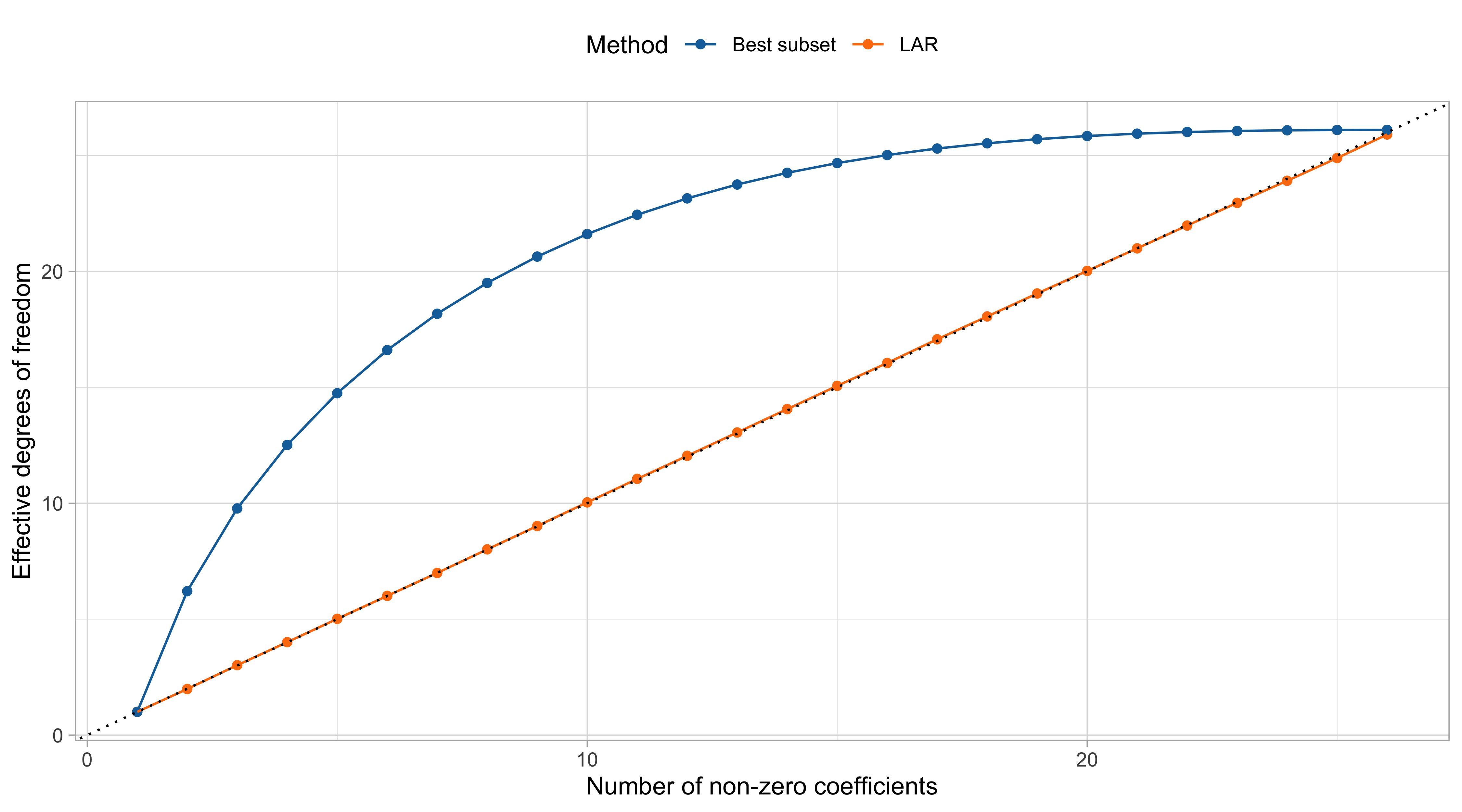
Effective degrees of freedom of LAR and best subset
Cross-validation for lasso
The LAR (lasso) estimate
Other properties of LAR and lasso
Bayesian interpretation: the penalty can be interpreted as a Laplace prior on \beta.
As mentioned, under certain conditions the LAR algorithm can be seen as the limiting case of a boosting procedure, in which small corrections to predictions are iteratively performed.
The nonnegative garrote (Breiman, 1995) is a two-stage procedure with a close relationship to the lasso. Breiman’s paper was the inspiration for Tibshirani (1996).
There is a large body of theoretical work on the behavior of the lasso, focused on:
- the mean-squared-error consistency of the lasso;
- the recovery of the nonzero support set of the true regression parameters, sometimes called sparsistency.
The interested reader may have a look at the (very technical) Chapter 11 of Hastie, Tibshirani and Wainwright (2015)
Summary of LARS and lasso
The prostate dataset. A summary of the estimates
| Least squares | Best subset | PCR | Ridge | Lasso | |
|---|---|---|---|---|---|
(Intercept) |
2.465 | 2.477 | 2.455 | 2.467 | 2.468 |
lcavol |
0.680 | 0.740 | 0.287 | 0.588 | 0.532 |
lweight |
0.263 | 0.316 | 0.339 | 0.258 | 0.169 |
age |
-0.141 | . | 0.056 | -0.113 | . |
lbph |
0.210 | . | 0.102 | 0.201 | . |
svi |
0.305 | . | 0.261 | 0.283 | 0.092 |
lcp |
-0.288 | . | 0.219 | -0.172 | . |
gleason |
-0.021 | . | -0.016 | 0.010 | . |
pgg45 |
0.267 | . | 0.062 | 0.204 | . |
The results on the test set
At the beginning of this unit, we split the data into training set and test set. Using the training, we selected \lambda via cross-validation or the C_p index.
Using the final test set with 30 observations, we will assess which model is preferable.
| OLS | Best subset | PCR | Ridge | Lasso | |
|---|---|---|---|---|---|
| Test error (MSE) | 0.521 | 0.492 | 0.496 | 0.496 | 0.48 |
All the approaches presented in this unit perform better than ordinary least squares.
The lasso is the approach with lowest mean squared error. At the same time, it is also a parsimonious choice.
Best subset is the second best, doing a good job in this example… but here p = 8, so there were no computational difficulties!
Elastic-net and pathwise algorithms
Elastic-net
- The elastic-net is a compromise between ridge and lasso. It selects variables like the lasso and shrinks together the coefficients of correlated predictors like ridge.
- Having removed the intercept, the elastic-net estimator \hat{\beta}_\text{en} is the minimizer of: \frac{1}{2n}\sum_{i=1}^n(y_i - \bm{x}_i^T\beta)^2 + \lambda\sum_{j=1}^p\left(\alpha |\beta_j| + \frac{(1 - \alpha)}{2}\beta_j^2\right), where 0 < \alpha < 1 and the complexity parameter \lambda > 0.
Ridge regression is a special case, when \alpha = 0. Lasso is also a special case, when \alpha = 1.
It is often not worthwhile to estimate \alpha using cross-validation. A typical choice is \alpha = 0.5.
An advantage of the elastic-net is that it has a unique solution, even when p > n.
Another nice property, shared by ridge, is that whenever \tilde{\bm{x}}_j = \tilde{\bm{x}}_\ell, then \hat{\beta}_{j,\text{en}} = \hat{\beta}_{\ell,\text{en}}. On the other hand, the lasso estimator would be undefined.
Convex optimization
- The estimators OLS, ridge, lasso, and elastic-net have a huge computational advantage compared, e.g., to best subset: they are all convex optimization problems.
- A function f: \mathbb{R}^p \rightarrow \mathbb{R} is convex if for any values \bm{b}_1, \bm{b}_2 \in \mathbb{R}^p and t \in [0, 1] it holds that f(t \bm{b}_1 + (1-t)\bm{b}_2) \le t f(\bm{b}_1) + (1-t) f(\bm{b}_2). Replacing \le with < for t \in(0,1) gives the definition of strict convexity.
- OLS and the lasso are, for a general design matrix \bm{X}, convex problems. On the other hand, ridge and elastic net are strictly convex, as well as OLS and lasso when \text{rk}(\bm{X}) = p.
Elastic-net with a single predictor
- The elastic-net estimate \hat{\beta}_\text{en} is typically obtained through the coordinate descent algorithm, which works well here due convexity and the following property.
- In the single-predictor scenario the elastic-net minimization problem simplifies to \hat{\beta}_\text{en} = \arg\min_{\beta}\frac{1}{2n}\sum_{i=1}^n(y_{i} - x_{i}\beta)^2 + \lambda \left( \alpha |\beta| + \frac{(1-\alpha)}{2} \beta^2\right).
- It can be shown that an explicit expression for \hat{\beta}_\text{en} is available, which is \hat{\beta}_\text{en} = \frac{1}{1 + (1 - \alpha)\lambda}\mathcal{S}_{\alpha\lambda}(\hat{\beta}_\text{ols}), where \mathcal{S}_\lambda(x) = \text{sign}(x)(|x| - \lambda)_+ is the soft-thresholding operator and the least square estimate is \hat{\beta}_\text{ols} = n^{-1}\sum_{i=1}^n x_i y_i.
Coordinate descent
The coordinate descent algorithm is based on a simple principle: optimize one coefficient (coordinate) at a time, keeping the others fixed.
We can re-write the objective function of the elastic-net in a more convenient form: \frac{1}{2n}\sum_{i=1}^n \left(\textcolor{red}{y_i - \sum_{k \neq j} x_{ik}\beta_k} - x_{ij} \beta_j\right)^2 + \lambda\left(\alpha |\beta_j| + \frac{(1 - \alpha)}{2} \beta_j^2\right) + \underbrace{\lambda \sum_{k\neq j}^p \{\alpha |\beta_k| + \frac{(1 - \alpha)}{2}\beta_k^2\}}_{\text{does not depend on } \beta_j},
- Let us define the partial residuals r_i^{(j)} = y_i - \sum_{k \neq j} x_{ik}\beta_k. Then the updated \beta_j is \beta_j \leftarrow \frac{1}{1 + (1 - \alpha)\lambda}\mathcal{S}_{\alpha\lambda}\left(\frac{1}{n}\sum_{i=1}^n x_{ij} r_i^{(j)}\right). We cycle this update for j=1,\dots,p, over and over until convergence.
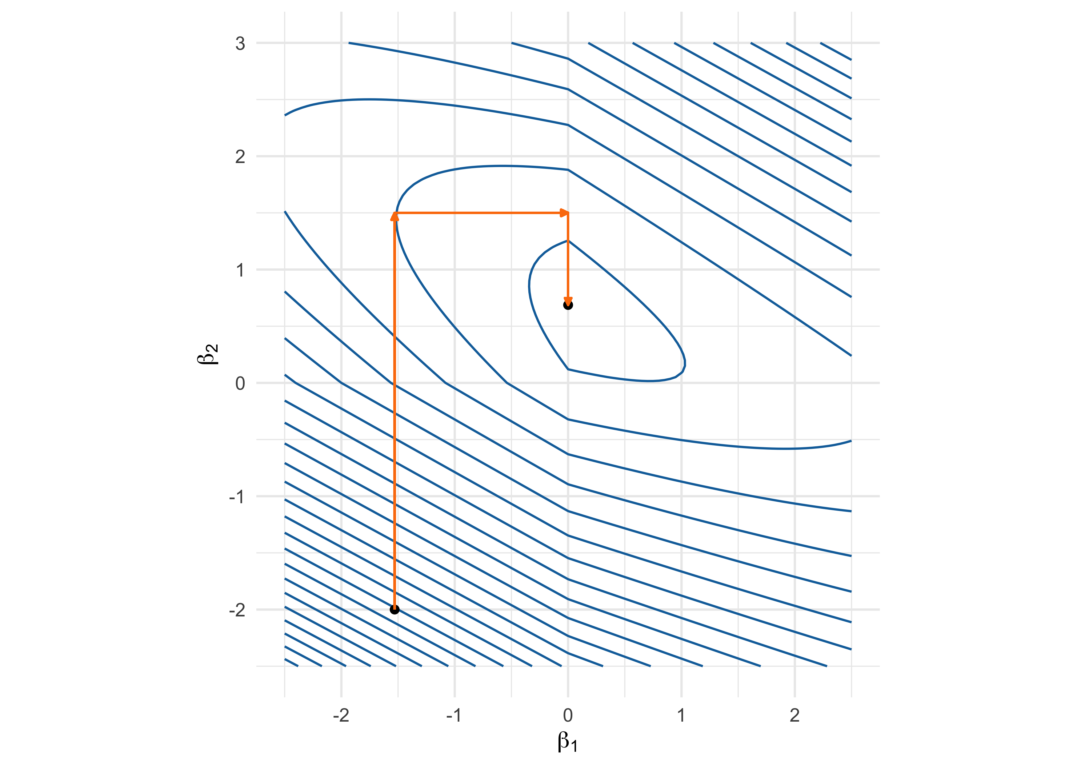
Coordinate descent - Example
Objective function: (1 - \beta_1 - 2 \beta_2)^2 + (3 - \beta_1 - 2 \beta_2)^2 + 5 (|\beta_1| + |\beta_2|).
Pathwise coordinate optimization
In a regression model with an elastic-net penalty, the coordinate descent is theoretically guaranteed to reach the global minimum.
The coordinate descent algorithm is implemented in the
glmnetpackage. It is, de facto, the default algorithm for penalized generalized linear models.The
glmnetimplementation is very efficient due to several additional tricks:- The warm start. The algorithm for \lambda_k is initialized at the previous solution using \lambda_{k-1}.
- Partial residuals can be efficiently obtained without re-computing the whole linear predictor.
- The code is written in C++ from version 4.1-3, it used to be written in Fortran.
- Many other tricks are employed: active set convergence, tools for sparse \bm{X} matrices, etc.
The same algorithm can also be used to fit ridge regression and lasso, which is often convenient even though alternatives would be available.
Generalized linear models
Generalized linear models
- Almost everything we discussed in this unit for regression problems can be extended to GLMs and, in particular, to classification problems.
Shrinkage methods for GLMs
Shrinkage methods such as ridge and lasso can also be generalized to GLMs.
The elastic-net approach for logistic regression, which covers ridge and lasso as special cases, becomes: \min_{(\beta_0, \beta)}\left\{ -\frac{1}{n}\sum_{i=1}^n y_i (\beta_0 + \bm{x}_i^T\beta) - \log\{1 + \exp(\beta_0 + \bm{x}_i^T\beta)\} + \lambda\sum_{j=1}^p\left(\alpha |\beta_j| + \frac{(1 - \alpha)}{2}\beta_j^2\right)\right\}, which is an instance of penalized log-likelihood.
Most of the properties (e.g. ridge = variance reduction and shrinkage, lasso = variable selection) and other high-level considerations we made so far are still valid.
Computations are somewhat more cumbersome. The
glmnetpackage provides the numerical routines for fitting this model, using variants of coordinate descent.The core idea is to obtain a quadratic approximation of the log-likelihood, as for IWLS. Then, the approximated loss becomes a (weighted) penalized regression problem.
References
References I
- Main references
- Chapter 3 of Azzalini, A. and Scarpa, B. (2011), Data Analysis and Data Mining, Oxford University Press.
- Chapters 3 and 4 of Hastie, T., Tibshirani, R. and Friedman, J. (2009), The Elements of Statistical Learning, Second Edition, Springer.
- Chapter 16 of Efron, B. and Hastie, T. (2016), Computer Age Statistical Inference, Cambridge University Press.
- Chapters 2,3 and 5 of Hastie, T., Tibshirani, R. and Wainwright, M. (2015). Statistical Learning with Sparsity: The Lasso and Generalizations. CRC Press.
- Best subset selection
- Hastie, T., Tibshirani, R., and Tibshirani, R.J. (2020). Best subset, forward stepwise or lasso? Analysis and recommendations based on extensive comparisons. Statistical Science 35(4): 579–592.
References II
- Ridge regression
- Hoerl, A. E., and Kennard, R. W. (1970). Ridge regression: biased estimation for nonorthogonal problems. Technometrics 12(1), 55–67.
- Hastie, T. (2020). Ridge regularization: an essential concept in data science. Technometrics, 62(4), 426-433.
- Lasso
- Tibshirani, R. (1996). Regression selection and shrinkage via the lasso. Journal of the Royal Statistical Society. Series B: Statistical Methodology, 58(1), 267-288.
- Efron, B., Hastie, T., Johnstone, I., and Tibshirani, R. (2004). Least Angle Regression. Annals of Statistics 32(2), 407-499.
- Zou, H., Hastie, T., and Tibshirani, R. (2007). On the ‘degrees of freedom’ of the lasso. Annals of Statistics 35(5), 2173-2192.
- Tibshirani, R. J. (2013). The lasso problem and uniqueness. Electronic Journal of Statistics 7(1), 1456-1490.
References III
- Elastic-net
- Zou, H. and Hastie, T. (2005). Regularization and variable selection via the elastic net. Journal of the Royal Statistical Society. Series B: Statistical Methodology 67(2), 301-320.
- Computations for penalized methods
- Friedman, J., Hastie, T., Höfling, H. and Tibshirani, R. (2007). Pathwise coordinate optimization. The Annals of Applied Statistics 1(2), 302-32.
- Tay, J. K., Narasimhan, B. and Hastie, T. (2023). Elastic net regularization paths for all generalized linear models. Journal of Statistical Software 106 (1).
Comments and computations
The correct way of doing cross-validation requires that the best subset selection is performed on every fold, possibly obtaining different “best” models with the same size.
Best subset selection is conceptually appealing, but it has a major limitation. There are \sum_{k=1}^p \binom{p}{k} = 2^p models to consider, which is computationally prohibitive!
There exist algorithms (i.e. leaps and bounds) that make this feasible for p \approx 30.
Recently, Bertsimas et al., 2016 proposed the usage of a mixed integer optimization formulation, allowing p to be in the order of hundreds.
Despite these advances, this problem remains computationally very expensive. See also the recent paper Hastie et al. (2020) for additional considerations and comparisons.