Introduction
Statistics III - CdL SSE
Homepage
“I would like to think of myself as a scientist, who happens largely to specialise in the use of statistics.”
Sir David Cox (1924-2022)
Statistica III is a monographic course on Generalized Linear Models (GLMs), a broadly applicable regression technique.
This is a B.Sc.-level course, but there are some prerequisites: it is assumed that you have already been exposed to:
- Simple linear regression, from Statistica I;
- Inferential statistics, from Statistica II;
- Linear models, from Analisi Statistica Multivariata and Econometria;
- R software, from Analisi Statistica Multivariata.
In Statistica III we extend linear models within a unified and elegant framework.
Regression is such an important topic that the tour will continue at the M.Sc. at CLAMSES. In Data Mining I will cover penalized methods and nonparametric regression.
Indeed, GLMs can be arguably regarded one of the most influential statistical ideas of the XX century.
Statistics of the 20th century
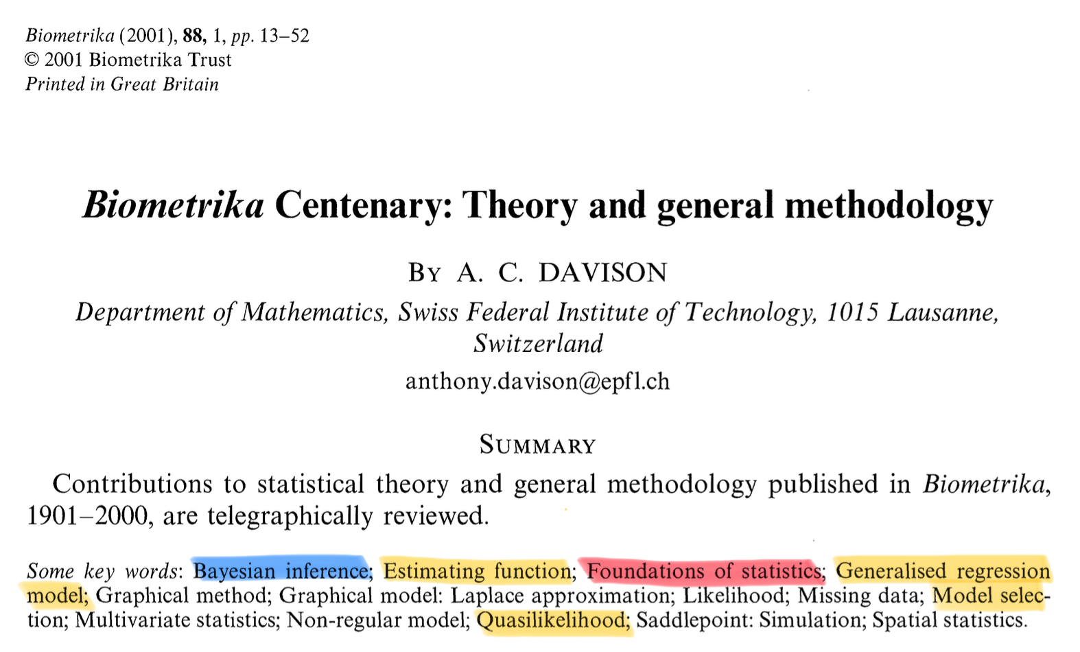
- Biometrika is among the most prestigious journals in Statistics. Past editors include Karl Pearson, Sir David Cox, and Anthony Davison.
Early ideas
Classical linear models and least squares began with the work of Gauss and Legendre who applied the method to astronomical data.
Their idea, in modern terms, was to predict the mean of a normal, or Gaussian, distribution as a function of a covariate: \mathbb{E}(Y_i) = \beta_1 + \beta_2 x_i, \qquad i=1,\dots,n.
As early as Fisher (1922), a more advanced non-linear model was introduced, designed to handle proportion data of the form S_i / m.
Through some modeling and calculus, Fisher derived a binomial model for S_i, with \mathbb{E}(S_i/m) = \pi_i = 1 - \exp\{-\exp(\beta_1 + \beta_2 x_i)\}, \qquad i = 1, \dots, n. where \pi_i \in (0, 1) is the probability of success of a binomial distribution.
The corresponding inverse relationship is known as the complementary log-log link function: \beta_1 + \beta_2 x_i = \log\{-\log(1-\pi_i)\}.
Early ideas II
- In the probit model, developed by Bliss (1935), a Binomial model for S_i is specified with \mathbb{E}(S_i/m) = \pi_i = \Phi(\beta_1 + \beta_2 x_i),\qquad i = 1, \dots, n. where \Phi(x) is the cumulative distribution function of a Gaussian distribution.
Dyke and Patterson (1952) also considered the case of modelling proportions, but specified \mathbb{E}(S_i/m) = \pi_i = \frac{\exp(\beta_1 + \beta_2 x_i)}{1 + \exp(\beta_1 + \beta_2 x_i)}, \qquad i = 1, \dots, n.
The corresponding inverse relationship is known as the logit link function: \beta_1 + \beta_2 x_i = \text{logit}(\pi_i) = \log\left(\frac{\pi_i}{1 - \pi_i}\right). In fact, this approach is currently known as logistic regression.
- See Chapter 1 of McCullagh and Nelder (1989) for a more exhaustive historical account, including early ideas about the Poisson distribution, the multinomial, and more.
Generalized linear models
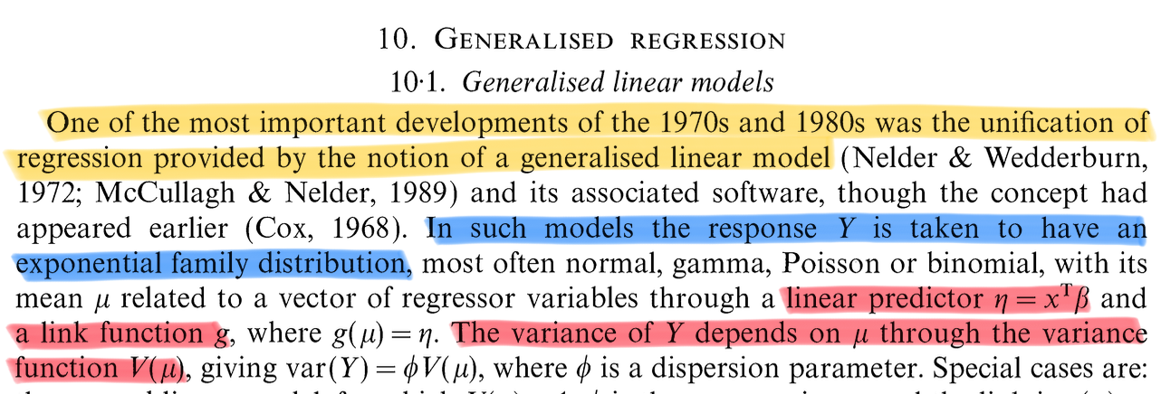
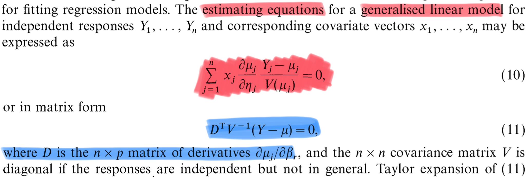
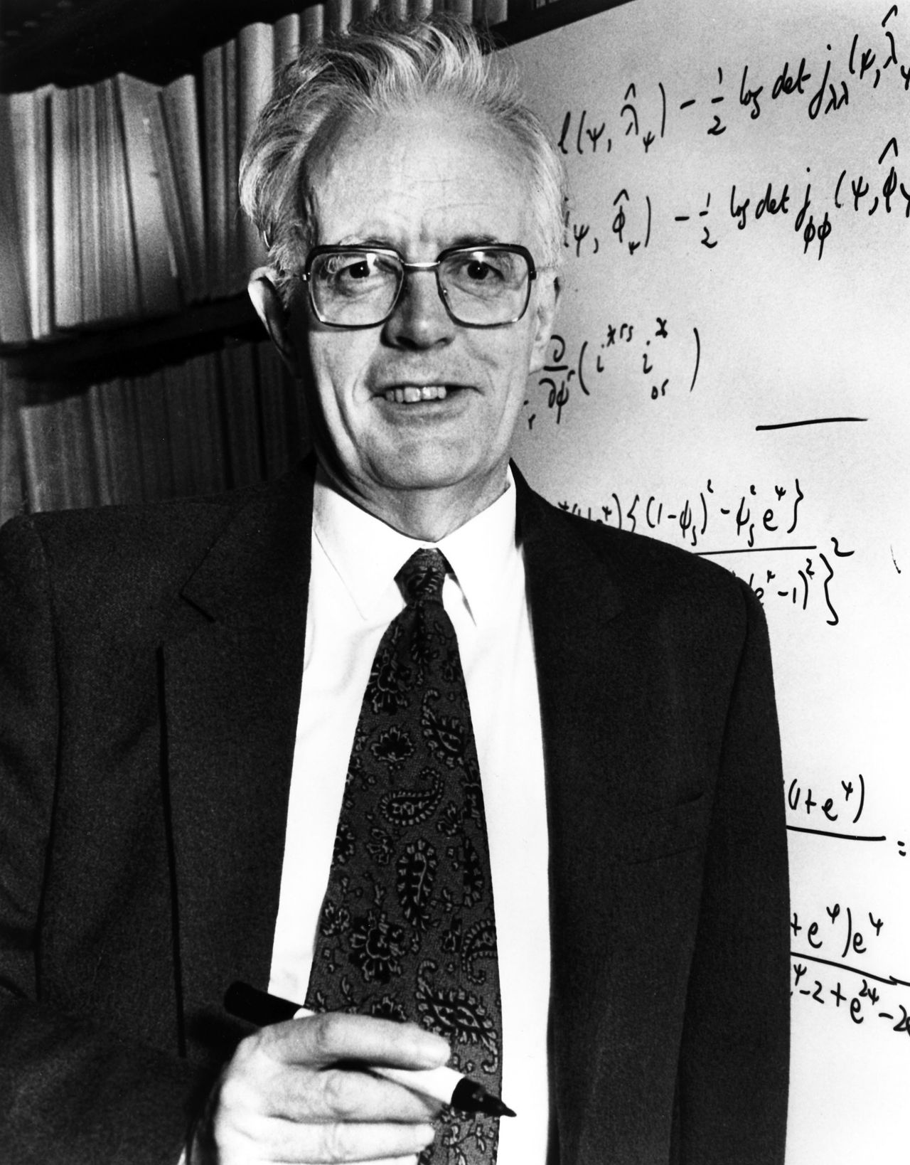
- The pivotal paper by Nelder and Wedderburn (1972) unified all these approaches.
Quasi likelihoods
The content of this course
- General theory
- Linear models and misspecification
- Generalized Linear Models (GLMs)
- Linear models and misspecification
- Notable models
- Binary and binomial regression
- Poisson regression
- Advanced topics
- Quasi likelihoods
- Unfortunately, due to time constraints, we will not cover:
- Contingency tables and log-linear models;
- Multinomial response and ordinal response models;
- Models with correlated responses (random effects);
- Nonparametric regression.
- These topics will be covered e.g. in Statistica Multivariata and Data Mining at CLAMSES.
Textbooks
We will use several textbooks throughout this course — some more specialized than others. They are listed in order of importance:
- The book by Salvan et al. (2020), in Italian, is the main textbook. Most of the material covered in these slides can be found there. I will also try to follow its notation as closely as possible.
- The book by Azzalini (2008), in Italian, is more concise but very enjoyable to read. I highly recommend browsing through it.
- The book by Agresti (2015), in English, is comprehensive and extremely well-written. It was the one I consulted most while preparing this course. Its only “drawback” is that it is in English.
- The book by McCullagh and Nelder (1989), in English, is an advanced and authoritative textbook intended for experienced statisticians (at least at the M.Sc. level). Feel free to explore it out of curiosity, but it is not a main reference.
Exam
- The written exam has two parts, held on the same day:
- Theory and exercises: questions to assess understanding of concepts and the ability to correctly set up a statistical model.
- Data set analysis: applied analysis of a dataset using R.
- Theory and exercises: questions to assess understanding of concepts and the ability to correctly set up a statistical model.
- The overall mark is the average of the two parts.
- You must pass both parts (each \geq 18).
- The oral exam is optional:
- Can be requested by the student or the teacher
- Final mark = average of written and oral marks
- Can be requested by the student or the teacher
- The exam is closed-book and closed-notes, except for the R scripts provided at the beginning of the test.