The curse of dimensionality
Data Mining - CdL CLAMSES
Università degli Studi di Milano-Bicocca
Homepage

“In view of all that we have said in the foregoing sections, the many obstacles we appear to have surmounted, what casts the pall over our victory celebration? It is the curse of dimensionality, a malediction that has plagued the scientist from the earliest days.”
Richard Bellman
In Unit C we explored linear predictive models for high-dimensional data (i.e. p is large).
In Unit D we explored nonparametric predictive models for univariate data, placing almost no assumptions on f(x).
Thus, the expectations are that this unit should cover models with the following features:
- High-dimensional, with large p;
- Nonparametric, placing no assumptions on f(\bm{x}).
The title of this unit, however, is not “fully flexible high-dimensional models.”
Instead, it sounds like bad news is coming. Let us see why, unfortunately, this will be indeed the case.
Multidimensional local regression
- At least conceptually, kernel methods could be applied with two or more covariates.
- To estimate f on a specific point \bm{x} = (x_1,\dots,x_p)^T, a natural extension of the Nadaraya-Watson takes the form \hat{f}(x) = \frac{1}{\sum_{i'=1}^n w_{i'}(\bm{x})}\sum_{i=1}^n w_i(\bm{x}) y_i = \sum_{i=1}^n s_i(\bm{x}) y_i, where the weights w_i(\bm{x}) are defined as w_i(\bm{x}) = \prod_{j=1}^p \frac{1}{h_j} w\left(\frac{x_{ij} - x_j}{h_j}\right).
This estimator is well-defined and it considers “local” points in p dimensions.
If the theoretical definition of multidimensional nonparametric tools is not a problem, why are they not used in practice?
The curse of dimensionality I
- When the function f(x) is entirely unspecified and a local nonparametric method is used, a dense dataset is needed to get a reasonably accurate estimate \hat{f}(x).
However, when p grows, the data points become sparse, even when n is “big” in absolute terms.
In other words, a neighborhood of a generic point x contains a small fraction of observations.
Thus, a neighborhood with a fixed percentage of data points is no longer local.
- To put it another way, to get a local neighborhood with 10 data points along each axis we need about 10^p data points.
- As a consequence, much larger datasets are needed even for moderate p, because the sample size n needs to grow exponentially with p.
The curse of dimensionality II
The following illustration may help clarify this notion of sparsity. Let us consider data points that are uniformly distributed on (0, 1)^p, that is \bm{x}_i \overset{\text{iid}}{\sim} \text{U}^p(0, 1).
Then, the median distance from the origin (0,\dots,0)^T to the closest point is: \text{dist}(p, n) = \left\{1 - \left(\frac{1}{2}\right)^{1/n}\right\}^{1/p}.
In the univariate case, such a median distance for n = 100 is quite small: \text{dist}(1, 100) = 0.007.
Conversely, when the dimension p increases, the median distance becomes: \text{dist}(2, 100) = 0.083, \quad \text{dist}(10, 100) = 0.608, \quad \text{dist}(50, 100) = 0.905. Note that we get \text{dist}(10, 1000) = 0.483 even with a much larger sample size.
Most points are close to the boundary, making predictions very hard.
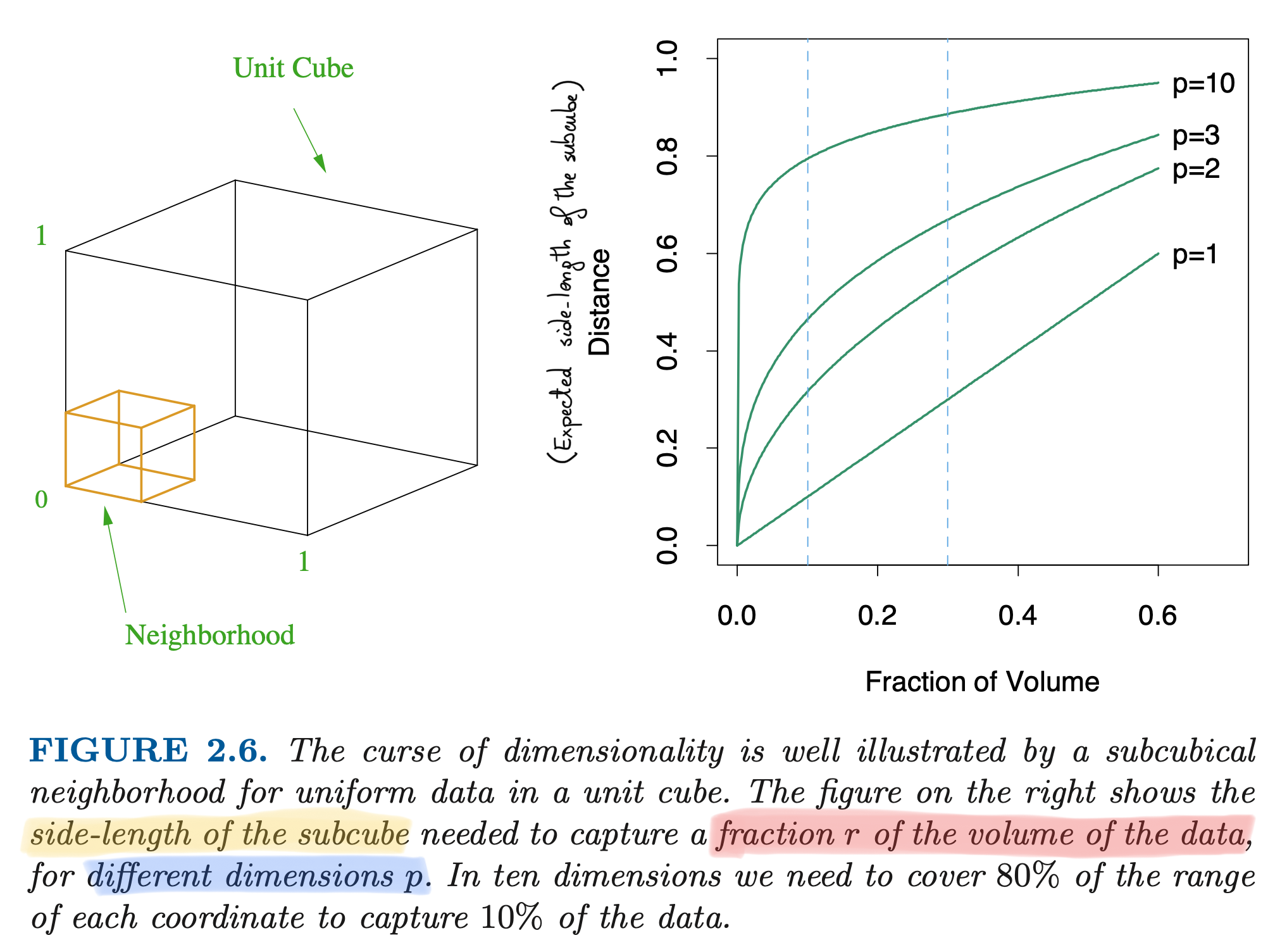
The curse of dimensionality III
The following argument gives another intuition of the curse of dimensionality. Let us consider again uniform covariates \bm{x}_i \overset{\text{iid}}{\sim} \text{U}^p(0, 1).
Let us consider a subcube which contains a fraction r \in (0, 1) of the total number of observations n. In the univariate case (p = 1), the side of this cube is r.
In the more general case, it can be shown that on average, the side of the cube is \text{side}(r, p) = r^{1/p}, which is again exponentially increasing in p.
Hence, when p = 1, the expected amount of points in the local sub-interval (0, 1/10) is again 1/10.
Instead, when p = 10 the number of points in the local subcube (0, 1)^{10} is n \left(\frac{1}{10}\right)^{10} = \frac{n}{1{,}000{,}000{,}000}.
The curse of dimensionality (HTF, 2011)
Implications of the curse of dimensionality
In the local kernel smoothing approach, we can precisely quantify the impact of the curse of dimensionality on the mean squared error.
Under some regularity conditions, the Nadaraya-Watson and the local linear regression estimator has asymptotic mean squared error \mathbb{E}\left[\{f(x) - \hat{f}(x)\}^2\right] \sim n^{-4/5}, which is slower than the parametric rate n^{-1}, but still reasonably fast for predictions.
Conversely, it can be shown that in high-dimension the asymptotic rate becomes \mathbb{E}\left[\{f(\bm{x}) - \hat{f}(\bm{x})\}^2\right] \sim n^{-4/(4 + p)}.
Thus, the sample size for a p-dimensional problem to have the same accuracy as a sample size n in one dimension is m \propto n^{c p}, with c = (4 + p)/(5p) > 0.
To maintain a given degree of accuracy of a local nonparametric estimator, the sample size must increase exponentially with the dimension p.
Escaping the curse
Is there a “solution” to the curse of dimensionality? Well, yes… and no.
If f(x) is assumed to be arbitrarily complex and our estimator f(x) is nonparametric, we are destined to face the curse.
However, in linear models you never encountered the curse of dimensionality. Indeed: \frac{1}{n}\sum_{i=1}^n\mathbb{E}\left\{(\bm{x}_i^T\beta - \bm{x}_i^T\hat{\beta})^2\right\} = \sigma^2\frac{p}{n}, which is increasing linearly in p, but not exponentially.
Linear models make assumptions and impose a structure. If the assumptions are correct, the estimates exploit global features and are less affected by the local sparsity.
Nature is not necessarily a linear model, so we explored the nonparametric case.
Nonetheless, making (correct) assumptions and therefore imposing (appropriate) restrictions is beneficial, to the extent that it is unavoidable in high dimensions.
Escaping the curse
The multidimensional methods you will study (GAM, trees, random forest, boosting, neural networks, etc.) deal with the curse of dimensionality by making (implicit) assumptions.
These assumptions differentiate because of:
- The particular nature of the knowledge they impose (e.g., no interactions, piecewise constant functions, etc.);
- The strength of this assumption;
- The sensitivity of the methods to a potential violation of the assumptions.
Thus, several alternative ideas and methods are needed; no single “best” algorithm exists.
This is why having a well-trained statistician on the team is important because they can identify the method that best suits the specific applied example.
…or at least, they will be aware of the limitations of the methods.
References
- Main references
- Section 4.3 of Azzalini, A. and Scarpa, B. (2011), Data Analysis and Data Mining, Oxford University Press.
- Section 2.5 of Hastie, T., Tibshirani, R., and Friedman, J. (2009), The Elements of Statistical Learning, Second Edition, Springer.
- Sections 4.5 and 5.12 of Wasserman, L. (2006), All of Nonparametric statistics, Springer.
