ABACO26
Nonparametric predictive inference for discrete data via Metropolis-adjusted Dirichlet sequences
Università degli Studi di Milano-Bicocca
2026-02-06
Warm thanks
Davide Agnoletto (Duke University)

David Dunson (Duke University)

Nonparametric modelling of count data
- Bayesian nonparametric modeling of counts distributions is a challenging task. Nonparametric mixtures of discrete kernels (Canale and Dunson 2011) can be cumbersome in practice.
- Alternatively, one could directly specify a DP prior on the data generator as Y_i\mid P \overset{\textup{iid}}{\sim} P,\quad P\sim\mathrm{DP}(\alpha, P_0), for Y_i\in\mathcal{Y}=\{0,1,\ldots\}, i=1,\ldots,n, where \alpha is the precision parameter and P_0 a base parametric distribution, such as a Poisson.
The Dirichlet process is mathematically convenient. However, the corresponding posterior lacks smoothing, which can lead to poor performance.
Within the hypothetical approach, it is unclear how to specify a nonparametric process with the same simplicity and flexibility as the DP prior while allowing for smoothing.
- Our proposal: a predictive sequence tailored to count data inspired by kernel density estimators.
Illustrative example I
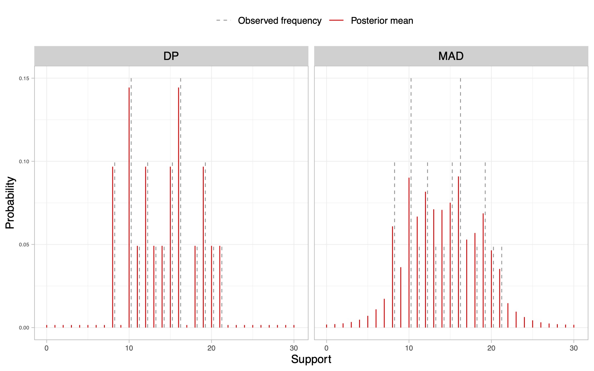
- Left plot: posterior mean of a DP. Right plot: posterior mean of the proposed MAD sequence.
Foundations
- De Finetti’s representation Theorem (De Finetti 1937) it provides the fundamental justification to the two approaches to Bayesian statistics: the hypothetical approach and the predictive approach.
De Finetti’s representation theorem
Let (Y_n)_{n\ge 1}, be a sequence of exchangeable random variables. Then there exists a unique probability measure \Pi such that, for any n\ge 1 and A_1,\dots,A_n \mathbb{P}(Y_1 \in A_1,\ldots,Y_n \in A_n) = \int_{\mathcal{P}} \prod_{i=1}^n p(A_i)\,\Pi(\mathrm{d}p).
- In a hierarchical formulation, we will say that (Y_n)_{n \ge 1} is exchangeable if and only if \begin{aligned} Y_i \mid P &\overset{\textup{iid}}{\sim} P, \qquad i \ge 1, \\ P &\sim \Pi, \end{aligned} where P is a random probability measure and \Pi is the prior law.
Hypothetical approach
The hypothetical approach represents the the most common way to operate within the Bayesian community.
In a parametric setting, \Pi has support on a class \Theta\subseteq\mathbb{R}^p with p<\infty, such that \boldsymbol{\theta}\in\Theta indexes the class of distributions \mathcal{P}_{\boldsymbol{\theta}}=\{P_{\boldsymbol{\theta}} : \boldsymbol{\theta} \in \Theta\subseteq\mathbb{R}^p\}.
Bayes’ rule takes the well-known formulation: \pi(\boldsymbol{\theta}\mid y_{1:n}) \propto \pi(\boldsymbol{\theta}) \prod_{i=1}^n p_{\boldsymbol{\theta}}(y_i), where \pi and p_{\boldsymbol{\theta}} denote the probability density functions associated with \Pi and P_{\boldsymbol{\theta}}, respectively.
However, when the link between observations and parameter of interest cannot be easily expressed through a distribution function, the traditional hypothetical approach fails.
Solution: generalized posterior distributions, sometimes called Gibbs-posteriors.
This is a lively recent topic, see for instance: Chernozhukov and Hong (2003); Bissiri et al. (2016) Heide et al. (2020); Grünwald and Mehta (2020); Knoblauch et al. (2022); Matsubara et al. (2022); Matsubara et al. (2023); Jewson and Rossell (2022); Rigon et al. (2023); Agnoletto et al. (2025).
Generalizations of the hypothetical approach
- Bissiri et al. (2016) showed that the generalized posterior \pi_\omega(\boldsymbol{\theta} \mid y_{1:n}) \propto \pi(\boldsymbol{\theta}) \exp\left\{ - \omega \sum_{i=1}^n \ell(\boldsymbol{\theta}; y_i) \right\}, is the only coherent update of the prior beliefs about \boldsymbol{\theta}^* = \arg\min_{\boldsymbol{\theta}\in\Theta} \int_{\mathcal{Y}} \ell(\boldsymbol{\theta}; y)\, F_0(\mathrm{d}y), where \ell(\boldsymbol{\theta}, y) is a loss function, \omega is the loss-scale, and F_0 is the unknown true sampling distribution.
Learning the loss scale \omega from the data is a delicate task. Assuming a prior for \omega can lead to degenerate estimates if not accompanied by additional adjustments to the loss function.
However, there are several solutions for its calibration: Holmes and Walker (2017); Lyddon et al. (2019); Syring and Martin (2019); Matsubara et al. (2023).
Predictive approach
- Taking a predictive approach, one can implicitly characterize the prior via de Finetti theorem by specifying the sequence of predictive distributions of an exchangeable sequence: P_n(A) := \mathbb{P}(Y_{n+1}\in A\mid y_{1:n}), \qquad n \ge 1. This leads to an exchangeable sequences iff the conditions in Fortini et al. (2000) are satisfied.
- Example: the predictive construction of a Dirichlet process prior is such that Y_1\sim P_0 and Y_{n+1}\mid y_{1:n}\sim P_n for n\ge 1, where P_n(A) = \frac{\alpha}{\alpha+n} P_0(A) + \frac{1}{\alpha+n}\sum_{i=1}^n\mathbb{1}(y_i\in A), for any measurable set A.
- The possibility of specifying a sequence of one-step-ahead predictive distributions is appealing:
- it bypasses direct elicitation of the prior;
- it explicitly connects prediction and inference (see the next slide);
Connecting inference and prediction I
The posterior P \mid y_{1:n} is usually obtained through Bayes theorem, but this is not the only way.
We can characterize both prior and posterior of P through the predictive distributions P_n, which indeed contains all the necessary information.
- If (Y_n)_{n \ge 1} is exchangeable, then the prior and posterior mean of P coincide with the predictive: P_0(A) = \mathbb{P}(Y_1\in A) = \mathbb{E}\{P(A)\}, \qquad P_n(A) = \mathbb{P}(Y_{n+1}\in A\mid y_{1:n}) = \mathbb{E}(P(A) \mid y_{1:n}), \qquad n \ge 1.
- A deeper result holds, which is a corollary of Finetti theorem (Fortini and Petrone 2012).
De Finetti’s representation theorem (predictive form)
Let (Y_n)_{n \ge 1} be an exchangeable sequence with predictive distributions (P_n)_{n \ge 1}. Then P_n converges weakly (a.s. \mathbb{P}) to a random probability measure P distributed according to \Pi as n \to \infty.
Connecting inference and prediction II
- In other words, the sequence of predictive distributions P_n converges to a random probability measure P with prior distribution \Pi. The source of randomness is the data
Y_1, Y_2, Y_3, \dots Intuitively, before observing the data, our predictions eventually reflect the prior.
Given y_{1:n}, the sequence P_{n+m} converges weakly (a.s. \mathbb{P}) as m \to \infty to a random probability measure with posterior distribution \Pi(\cdot \mid y_{1:n}). The source of randomness is the future data
Y_{n+1}, Y_{n+2}, Y_{n+3}, \dots .This provides a natural alternative interpretation of the posterior distribution P \mid y_{1:n} and a practical algorithm for sampling from it, called predictive resampling.
Intuitively, posterior uncertainty arises from lack of knowledge about future observations. If we knew them, the posterior would collapse to a point mass (Bayesian consistency).
- This reasoning is at the heart of martingale posteriors (Fong et al. 2023).
Generalizations of the predictive approach
- Defining a sequence of predictive laws P_n that guarantees exchangeability—i.e., satisfies the two-step-ahead conditions of Fortini et al. (2000)—is a difficult task in practice.
Solution: replace exchangeability with the weaker requirement that (Y_n)_{n\ge1} is conditionally identically distributed (CID), also known as martingale posteriors.
The CID condition requires \mathbb{P}(Y_{n+k} \in \cdot \mid y_{1:n}) = \mathbb{P}(Y_{n+1} \in \cdot \mid y_{1:n}) = P_n(\cdot), \qquad \text{for all} \quad k \ge 1, \; n \ge 1. It is sufficient to verify this condition for k = 1 in order to ensure its validity for all k \ge 1.
Equivalently, Fong et al. (2023) express the above condition in a way that emphasizes the martingale property of the predictive distributions \mathbb{E}\{P_{n+1}(\cdot) \mid y_{1:n}\} = P_n(\cdot), \qquad n \ge 1.
A recursive predictive rule
- Intuitively, a better estimator would be obtained by replacing the indicator \mathbb{1}(\cdot) of the DP predictive scheme with a kernel that allows the borrowing of information between nearby values.
Let Y_1\sim P_0 and Y_{n+1} \mid y_{1:n} \sim P_n for n\ge 1, and let K_n(\cdot \mid y_n) be a sequence of transition kernels. We define the predictive distribution recursively: P_n(\cdot) = \mathbb{P}(Y_{n+1}\in \cdot\mid y_{1:n}) = (1-w_n) P_{n-1}(\cdot) + w_n K_{n}(\cdot\mid y_n), \qquad n \ge 1, where (w_n)_{n\ge1} are decreasing weights such that w_n\in(0,1), \sum_{n\ge1}w_n = \infty, and \sum_{n\ge1}w_n^2<\infty.
The choice of weights w_n = (\alpha +n)^{-1} gives the following DP-like predictive rule P_n(\cdot) = \frac{\alpha}{\alpha + n} P_0(\cdot) + \frac{1}{\alpha + n}\sum_{i=1}^nK_i(\cdot\mid y_i). Hence, the predictive law of a DP is a special case whenever K_i(\cdot \mid y_i) = \delta_{y_i}(\cdot).
The above sequence, beyond the DP special case, is not exchangeable and it will depend on the order of the data. Moreover, without further restrictions, is not necessarily CID!
Metropolis-adjusted Dirichlet (MAD) sequences
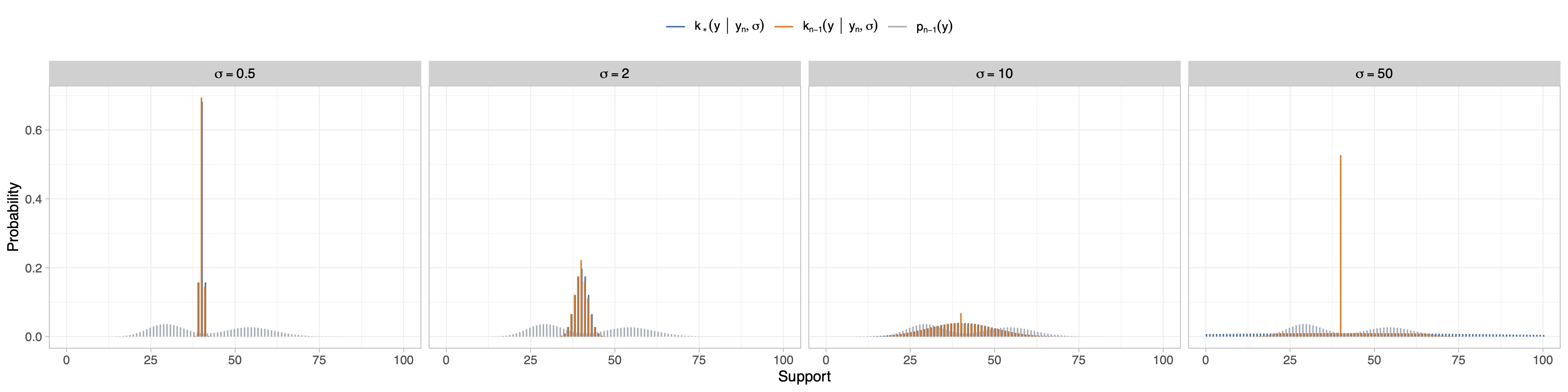
We assume that K_{n}(\cdot\mid y_n) is a Metropolis-Hastings kernel centered in y_n having pmf: k_{n}(y\mid y_n) = \gamma_{n}(y,y_n) k_*(y\mid y_n) + \mathbb{1}(y=y_n)\Big[\sum_{z\in\mathcal{Y}}\big\{1-\gamma_{n}(z,y_n)\big\}k_*(z\mid y_n)\Big], with acceptance probability \gamma_{n}(y,y_n) = \gamma(y, y_n, P_{n-1}) = \min\left\{1,\frac{p_{n-1}(y) k_*(y_n\mid y)}{p_{n-1}(y_n) k_*(y\mid y_n)}\right\}, where p_{n-1} is the probability mass functions associated to P_{n-1} and k_*(\cdot\mid y_n) is the pmf of a discrete base kernel centered at y_n.
We refer to P_n above as the Metropolis-adjusted Dirichlet (MAD) distribution with weights (w_n)_{n\ge1}, base kernel k_* and initial distribution P_0. We call (Y_n)_{n \ge 1} a MAD sequence.
Theorem (Agnoletto, R. and Dunson, 2025)
Let (Y_n)_{n\ge1} be a MAD sequence. Then, for every set of weights (w_n)_{n \ge 1}, discrete base kernel k_*, and initial distribution P_0, the sequence (Y_n)_{n\ge1} is conditionally identically distributed (CID).
Bayesian properties of CID sequences I
Corollary (Aldous 1985; Berti et al. 2004)
Consider a MAD sequence (Y_n)_{n\ge1}. Then, \mathbb{P}-a.s.,
(a) The sequence is asymptotically exchangeable, that is (Y_{n+1}, Y_{n+2}, \ldots) \overset{\textup{d}}{\longrightarrow} (Z_1, Z_2, \ldots), \qquad n \rightarrow \infty, where (Z_1,Z_2,\ldots) is an exchangeable sequence with directing random probability measure P;
(b) the corresponding sequence of predictive distributions (P_n)_{n\ge1} weakly converge to a random probability measures P (a.s. \mathbb{P}).
An asymptotic equivalent of de Finetti’s theorem holds: each MAD sequence has a corresponding unique prior on P.
The ordering dependence will vanish asymptotically and, informally, Y_i \mid P \overset{\mathrm{iid}}{\sim} P for large n.
The random probability measure P exists and is defined as the limit of the predictive distributions. However, it is not available explicitly.
Bayesian properties of CID sequences II
Corollary (Aldous 1985; Berti et al. 2004)
Let \theta = P(f) = \sum_{y \in \mathcal{Y}} f(y) p(y) and analogously \theta_n = P_n(f) = \sum_{y \in \mathcal{Y}} f(y) p_n(y) be any functional of interest. Consider a MAD sequence (Y_n)_{n\ge1}.
Then, \mathbb{P}-a.s., for every n\ge1 and every integrable function f:\mathcal{Y}\rightarrow\mathbb{R}, we have \mathbb{E}(\theta \mid y_{1:n}) = \mathbb{E}\{P(f) \mid y_{1:n}\} = P_n(f) = \theta_n
Broadly speaking, the posterior mean of any functional of interest of P coincides with the functional of the predictive.
Moreover, \mathbb{E}\{P(f)\}= P_0(f) = \theta_0 for every integrable function f, so that P_0 retains the role of a base measure as for standard Dirichlet sequences, providing an initial guess at P.
- Uncertainty quantification for \theta=P(f) is carried out by predictive resampling (Fong et al. 2023).
Predictive resampling for MAD sequences
Algorithm (Fortini and Petrone 2020):
- Compute P_n(\cdot) from the observed data y_{1:n}
- Set N\gg n
- For j = 1,\ldots,B
- For i=n+1,\ldots,N
- Sample Y_i\mid y_{1:i-1}\sim P_{i-1}
- Update P_i(\cdot) = (1-w_i)P_{i-1}(\cdot) + w_i K_{i-1}(\cdot\mid y_i)
- End For
- For i=n+1,\ldots,N
- End For
- Return P_N^{(1)}(\cdot),\ldots,P_N^{(B)}(\cdot), an iid sample from the distribution of P_N(\cdot)\mid y_{1:n}
On the choice of the base kernel
- In principle, any discrete distribution can be chosen as the base kernel k_*. However, it is natural to consider choices that allow the kernel to be centered at y_n while permitting control over the variance.
- We consider a rounded Gaussian distribution centered in y_n, with pmf k_*(y\mid y_n, \sigma) = \frac{\int_{y-1/2}^{y+1/2}\mathcal{N}(t\mid y_n, \sigma^2) \mathrm{d}t}{\sum_{z\in\mathcal{Y}} \int_{z-1/2}^{z+1/2}\mathcal{N}(t\mid y_n, \sigma^2) \mathrm{d}t}, for n\ge1, where \mathcal{N}(\cdot\mid y_n,\sigma^2) denotes a normal density function with mean y_n and variance \sigma^2.
Uncertainty quantification and calibration
- It can be shown that the asymptotic distribution of P(A)\mid y_{1:n} is \mathcal{N}(P_n(A), \Sigma_n r_n^{-1}) for n large, where the variance is \Sigma_n r_n^{-1} \approx \mathbb{E}\{[P_{n+1}(A)-P_n(A)]^2\mid y_{1:n}\}\sum_{k>n+1}w_k^2.
Weights that decay to zero quickly induce fast learning and convergence to the asymptotic exchangeable regime.
However, small values of w_n leads to underestimation of the posterior variability.
In practice, possible choices are w_n=(\alpha+n)^{-1} (i.e. DP-like sequence), w_n=(\alpha+n)^{-2/3} (Martin and Tokdar 2009), and w_n=(2 - n^{-1})(n+1)^{-1} (Fong et al. 2023).
We consider adaptive weights that we found have good empirical properties: w_n=(\alpha+n)^{-\lambda_n}, \qquad \lambda_n=\lambda+(1+\lambda)\exp\bigg\{-\frac{1}{N_*}n\bigg\}, with \lambda\in(0.5,1], N_*>0.
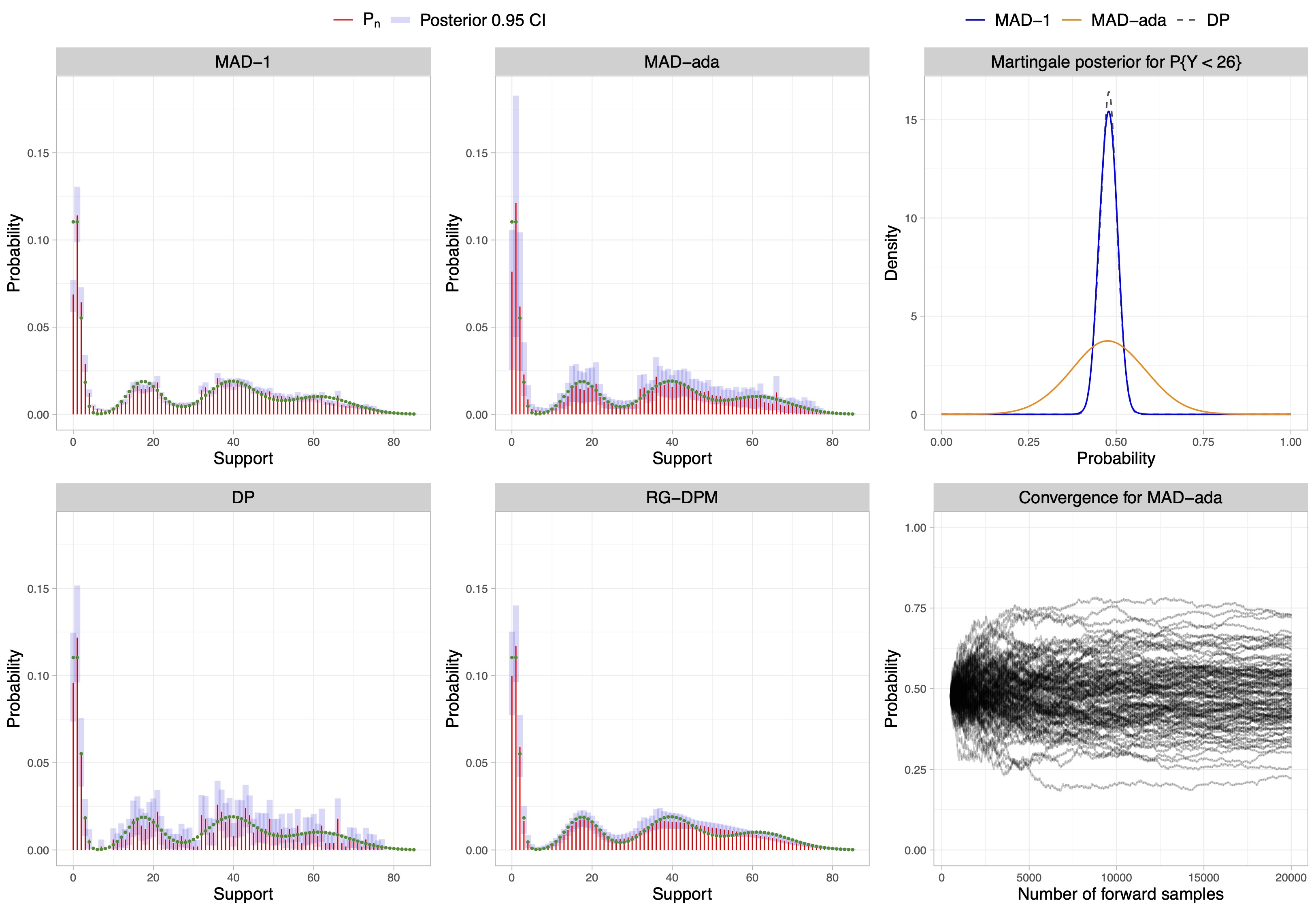
Illustrative examples II
Multivariate count and binary data
Extending MAD sequences for multivariate data is straightforward using a factorized base kernel k_*(\bm y\mid\bm y_n) = \prod_{j=1}^d k_*(y_j\mid y_{n,j}), with \bm y=(y_1,\ldots,y_d) and \bm y_n=(y_{n,1},\ldots,y_{n,d}).
In particular, MAD sequences can be employed for modeling multivariate binary data using an appropriate base kernel.
A natural step further is to use MAD sequences for nonparametric regression and classification.
Multivariate MAD sequences do not depend on the ordering of the variables, unlike most other martingale posteriors.
Simulations I
Out-of-sample prediction accuracy evaluated in terms of MSE and AUC for regression and classification, respectively, in specific simulation studies.
| Regress. (MSE) | Classific. (AUC) | ||||
|---|---|---|---|---|---|
| n=40 | n=80 | n=150 | n=300 | ||
| GLM | 120.77 [51.51] | 94.93 [8.37] | 0.796 [0.014] | 0.809 [0.007] | |
| BART | 101.17 [12.69] | 74.17 [10.00] | 0.863 [0.026] | 0.932 [0.009] | |
| RF | 99.98 [7.45] | 87.75 [6.53] | 0.882 [0.025] | 0.913 [0.015] | |
| DP | 1450.21 [5.53] | 1395.61 [8.72] | 0.644 [0.011] | 0.724 [0.012] | |
| MAD-1 | 91.07 [10.35] | 73.96 [7.60] | 0.873 [0.014] | 0.899 [0.008] | |
| MAD-2/3 | 88.83 [13.00] | 73.18 [9.58] | 0.869 [0.015] | 0.899 [0.009] | |
| MAD-DPM | 87.41 [12.36] | 72.07 [9.48] | 0.872 [0.014] | 0.901 [0.008] | |
| MAD-ADA | 90.61 [10.28] | 73.45 [7.69] | 0.874 [0.014] | 0.900 [0.008] |
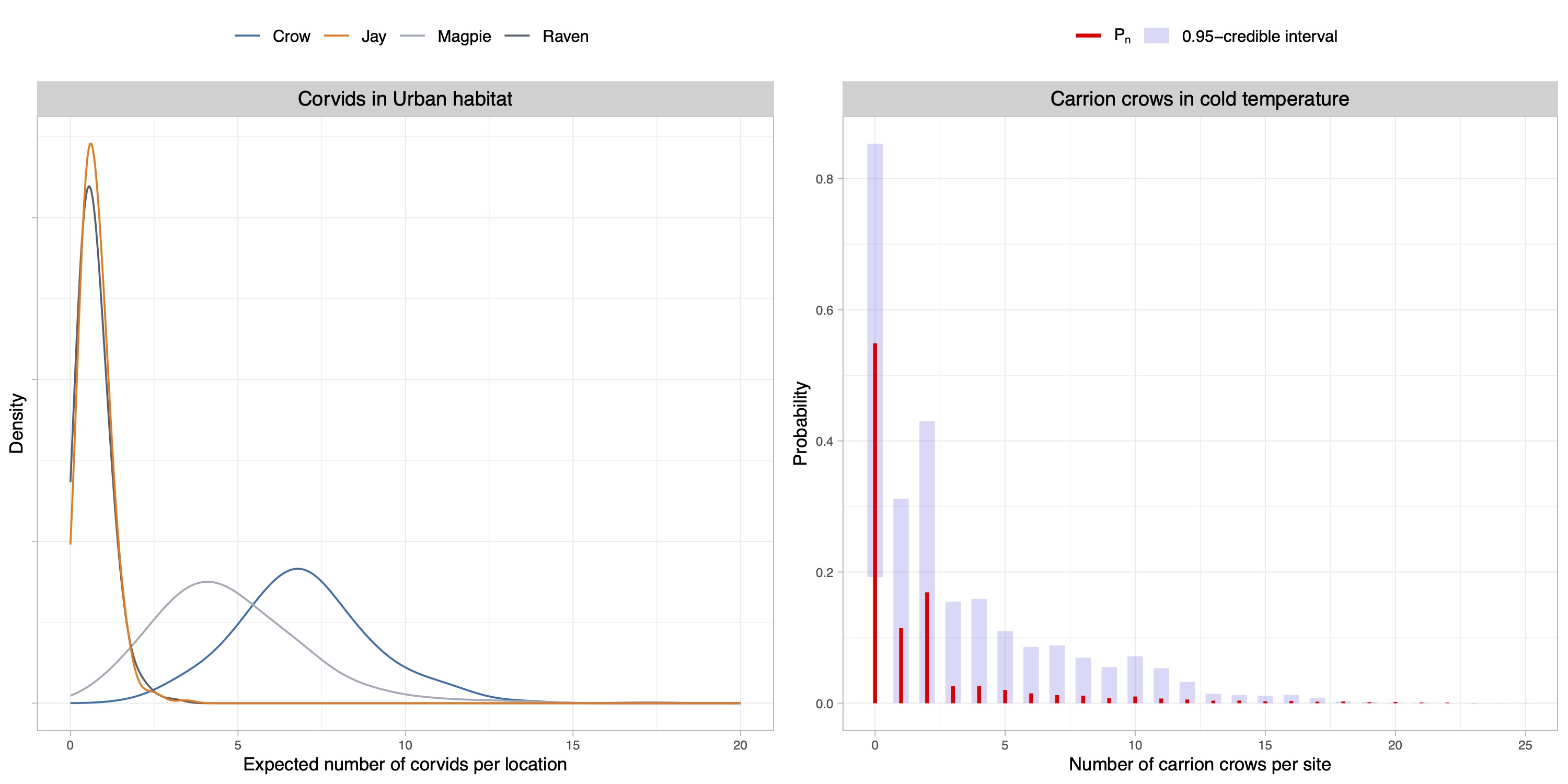
Application
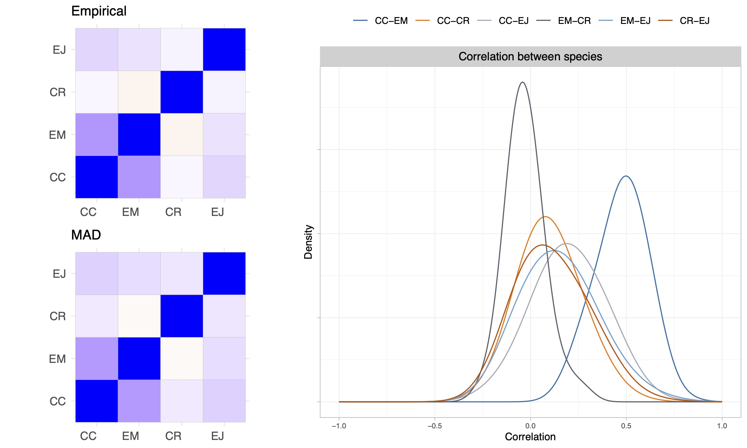
- We analyze the occurrence rates of 4 species corvids in Finland in year 2009 across different temperatures and habitats.
Application II
Thank you!

The main paper is:
Agnoletto, D., Rigon, T., and Dunson D.B. (2025+). Nonparametric predictive inference for discrete data via Metropolis-adjusted Dirichlet sequences. arXiv:2507.08629