Bayesian computations

Laplace approximation, Variational Bayes, Expectation Propagation

Author

Affiliation

Tommaso Rigon

DEMS

This unit discusses several approximate Bayesian methods presented in the slides of unit D.2. We will make use of the Pima Indian dataset again, as in the previous Markdown document B.1 and Markdown document B.2. Importantly, note that in this document, we will not standardize the predictors to make the computational problem more challenging.

The Pima Indian dataset

Pima <- rbind(MASS::Pima.tr, MASS::Pima.te)
y <- as.numeric(Pima$type == "Yes") # Binary outcome
X <- cbind(1, model.matrix(type ~ . - 1, data = Pima)) # Design matrix

We will employ a relatively vague prior centered at 0, namely \beta \sim N(0, 100 I_p).

B <- diag(10, ncol(X)) # Prior covariance matrix
b <- rep(0, ncol(X)) # Prior mean

The gold standard: MCMC

To assess the accuracy of the approximations, we first obtain a large number of posterior samples using the Pólya-gamma data augmentation approach. This is the code reported in the last paragraph of the Markdown document B.2.

library(BayesLogit)
logit_Gibbs <- function(R, burn_in, y, X, B, b) {
  p <- ncol(X)
  n <- nrow(X)
  out <- matrix(0, R, p) # Initialize an empty matrix to store the values

  P <- solve(B) # Prior precision matrix
  Pb <- P %*% b # Term appearing in the Gibbs sampling

  Xy <- crossprod(X, y - 1 / 2)

  # Initialization
  beta <- rep(0, p)

  # Iterative procedure
  for (r in 1:(R + burn_in)) {

    # Sampling the Pólya-gamma latent variables
    eta <- c(X %*% beta)
    omega <- rpg.devroye(num = n, h = 1, z = eta)

    # Sampling beta
    eig <- eigen(crossprod(X * sqrt(omega)) + P, symmetric = TRUE)

    Sigma <- crossprod(t(eig$vectors) / sqrt(eig$values))
    mu <- Sigma %*% (Xy + Pb)

    A1 <- t(eig$vectors) / sqrt(eig$values)
    beta <- mu + c(matrix(rnorm(1 * p), 1, p) %*% A1)

    # Store the values after the burn-in period
    if (r > burn_in) {
      out[r - burn_in, ] <- beta
    }
  }
  out
}

set.seed(123)

# Running the MCMC
fit_MCMC <- logit_Gibbs(R = 10^5, burn_in = 5000, y, X, B, b) # MCMC (gold standard)

Laplace approximation

The first approach considered is the Laplace approximation. The MAP is obtained using the Pólya-gamma data-augmentation, ensuring a monotonic procedure. Refer to the slides of unit D.2 for further details.

logit_Laplace <- function(y, X, B, b, tol = 1e-16, maxiter = 10000) {
  P <- solve(B) # Prior precision matrix
  Pb <- P %*% b # Term appearing in the Gibbs sampling

  logpost <- numeric(maxiter)
  Xy <- crossprod(X, y - 0.5)

  # Initialization
  beta <- solve(crossprod(X / 4, X) + P, Xy + Pb)
  eta <- c(X %*% beta)
  w <- tanh(eta / 2) / (2 * eta)
  w[is.nan(w)] <- 0.25

  # First value of the likelihood
  logpost[1] <- sum(y * eta - log(1 + exp(eta))) - 0.5 * t(beta) %*% P %*% beta

  # Iterative procedure
  for (t in 2:maxiter) {
    beta <- solve(qr(crossprod(X * w, X) + P), Xy + Pb)
    eta <- c(X %*% beta)
    w <- tanh(eta / 2) / (2 * eta)
    w[is.nan(w)] <- 0.25

    logpost[t] <- sum(y * eta - log(1 + exp(eta))) - 0.5 * t(beta) %*% P %*% beta

    if (logpost[t] - logpost[t - 1] < tol) {
      prob <- plogis(eta)
      return(list(
        mu = c(beta), Sigma = solve(crossprod(X * prob * (1 - prob), X) + P),
        Convergence = cbind(Iteration = (1:t) - 1, logpost = logpost[1:t])
      ))
    }
  }
  stop("The algorithm has not reached convergence")
}

The marginal densities of the first two regression coefficients and the “gold standard” obtained from the MCMC samples are reported.

library(tictoc)

tic()
fit_Laplace <- logit_Laplace(y, X, B, b)
toc()

0.015 sec elapsed

par(mfrow = c(1, 2))
plot(density(fit_MCMC[, 1]), xlab = expression(beta[1]), lty = "dotted", main = "")
curve(dnorm(x, fit_Laplace$mu[1], sqrt(fit_Laplace$Sigma[1, 1])), add = T)

plot(density(fit_MCMC[, 2]), xlab = expression(beta[2]), lty = "dotted", main = "")
curve(dnorm(x, fit_Laplace$mu[2], sqrt(fit_Laplace$Sigma[2, 2])), add = T)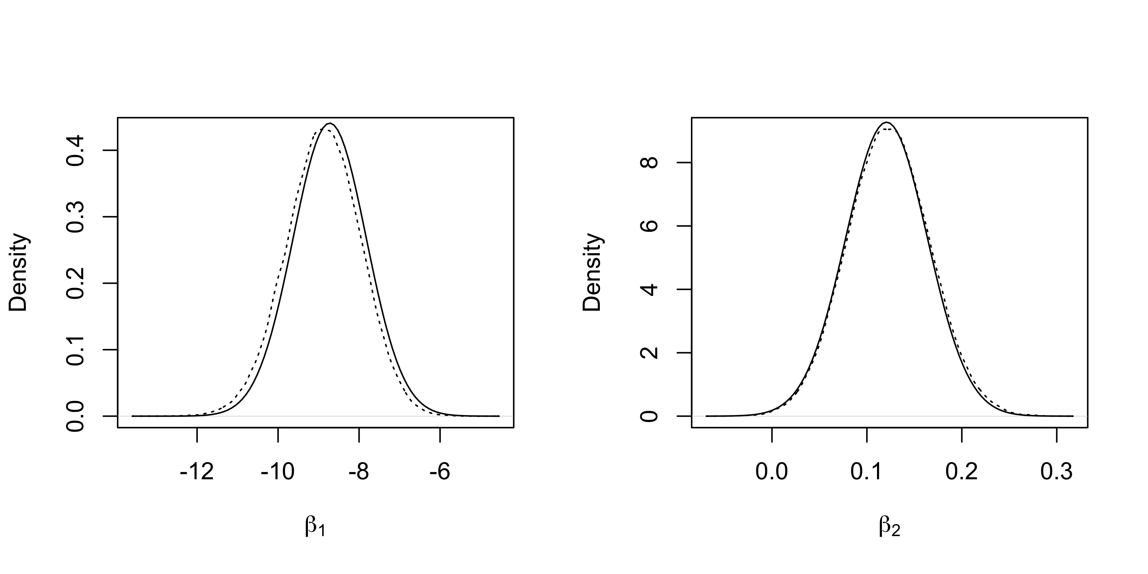

Variational Bayes

The second approximation is the Variational Bayes approximation of Jaakkola and Jordan (2000) and later considered also by Durante and Rigon (2019).

# Compute the log-determinant of a matrix
ldet <- function(X) {
  if (!is.matrix(X)) {
    return(log(X))
  }
  determinant(X, logarithm = TRUE)$modulus
}

logit_CAVI <- function(y, X, B, b, tol = 1e-16, maxiter = 10000) {
  lowerbound <- numeric(maxiter)
  p <- ncol(X)
  n <- nrow(X)

  P <- solve(B)
  Pb <- c(P %*% b)
  Pdet <- ldet(P)

  # Initialization for omega equal to 0.25
  P_vb <- crossprod(X * rep(1 / 4, n), X) + P
  Sigma_vb <- solve(P_vb)
  mu_vb <- Sigma_vb %*% (crossprod(X, y - 0.5) + Pb)
  eta <- c(X %*% mu_vb)
  xi <- sqrt(eta^2 + rowSums(X %*% Sigma_vb * X))
  omega <- tanh(xi / 2) / (2 * xi)
  omega[is.nan(omega)] <- 0.25

  lowerbound[1] <- 0.5 * p + 0.5 * ldet(Sigma_vb) + 0.5 * Pdet - 0.5 * t(mu_vb - b) %*% P %*% (mu_vb - b) + sum((y - 0.5) * eta + log(plogis(xi)) - 0.5 * xi) - 0.5 * sum(diag(P %*% Sigma_vb))

  # Iterative procedure
  for (t in 2:maxiter) {
    P_vb <- crossprod(X * omega, X) + P
    Sigma_vb <- solve(P_vb)
    mu_vb <- Sigma_vb %*% (crossprod(X, y - 0.5) + Pb)

    # Update of xi
    eta <- c(X %*% mu_vb)
    xi <- sqrt(eta^2 + rowSums(X %*% Sigma_vb * X))
    omega <- tanh(xi / 2) / (2 * xi)
    omega[is.nan(omega)] <- 0.25

    lowerbound[t] <- 0.5 * p + 0.5 * ldet(Sigma_vb) + 0.5 * Pdet - 0.5 * t(mu_vb - b) %*% P %*% (mu_vb - b) + sum((y - 0.5) * eta + log(plogis(xi)) - 0.5 * xi) - 0.5 * sum(diag(P %*% Sigma_vb))

    if (abs(lowerbound[t] - lowerbound[t - 1]) < tol) {
      return(list(
        mu = c(mu_vb), Sigma = matrix(Sigma_vb, p, p),
        Convergence = cbind(
          Iteration = (1:t) - 1,
          Lowerbound = lowerbound[1:t]
        ), xi = xi
      ))
    }
  }
  stop("The algorithm has not reached convergence")
}

The marginal densities of the first two regression coefficients and the “gold standard” obtained from the MCMC samples are reported.

tic()
fit_CAVI <- logit_CAVI(y, X, B, b)
toc()

0.034 sec elapsed

par(mfrow = c(1, 2))
plot(density(fit_MCMC[, 1]), xlab = expression(beta[1]), lty = "dotted", main = "", ylim = c(0, 0.6))
curve(dnorm(x, fit_CAVI$mu[1], sqrt(fit_CAVI$Sigma[1, 1])), add = T)

plot(density(fit_MCMC[, 2]), xlab = expression(beta[2]), lty = "dotted", main = "", ylim = c(0, 12))
curve(dnorm(x, fit_CAVI$mu[2], sqrt(fit_CAVI$Sigma[2, 2])), add = T)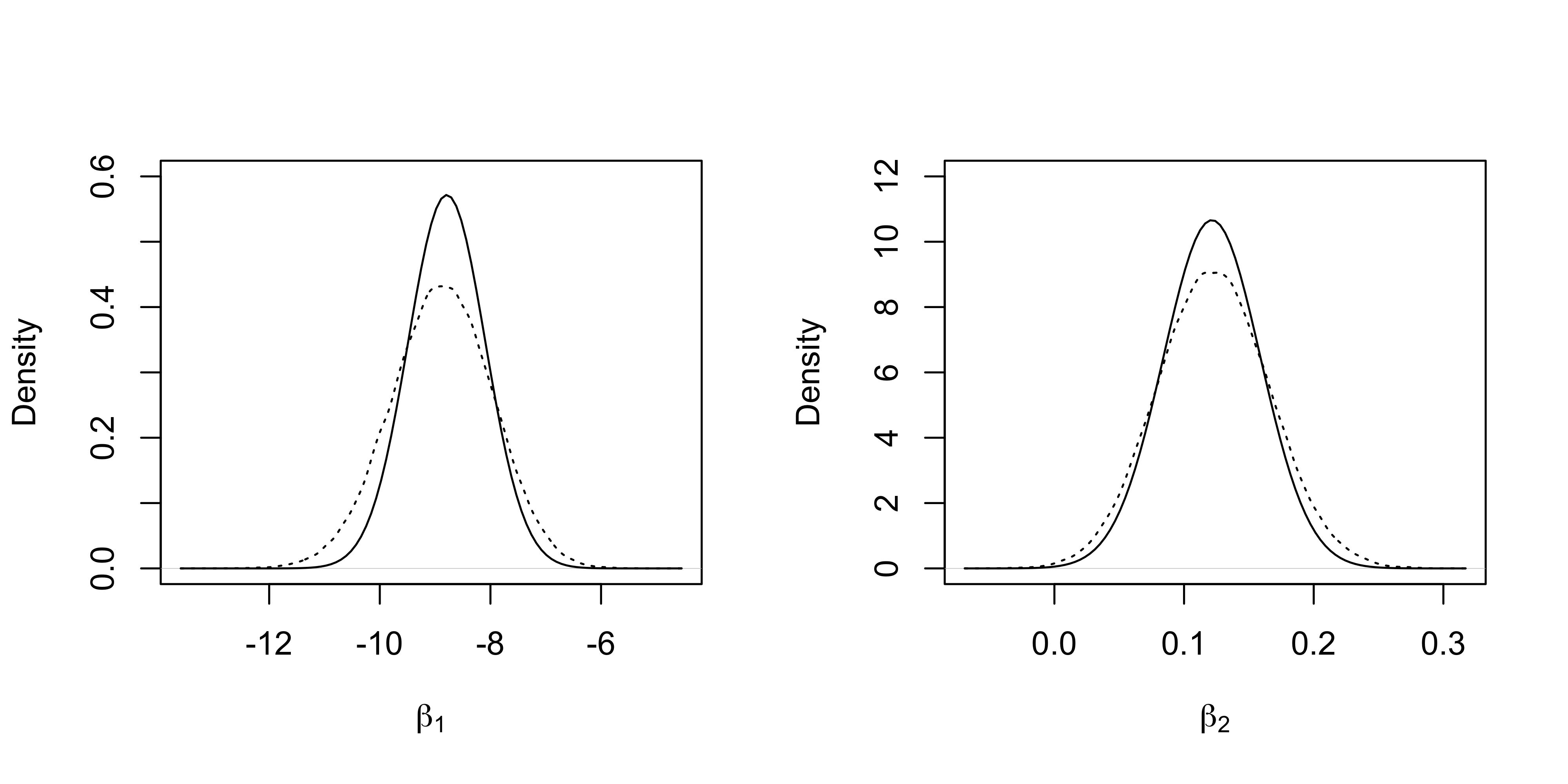

Hybrid Laplace

The fourth approach is based on the variational Bayes approximation mean estimate plugged into the Fisher information matrix. This procedure is not described in the slides of unit D.2.

logit_HL <- function(y, X, B, b, tol = 1e-16, maxiter = 10000) {
  fit_HL <- logit_CAVI(y, X, B, b, tol, maxiter)
  prob <- c(plogis(X %*% fit_CAVI$mu))
  fit_HL$Sigma <- solve(crossprod(X * prob * (1 - prob), X) + solve(B))
  fit_HL
}

The marginal densities of the first two regression coefficients and the “gold standard” obtained from the MCMC samples are reported.

fit_HL <- logit_HL(y, X, B, b)

par(mfrow = c(1, 2))
plot(density(fit_MCMC[, 1]), xlab = expression(beta[1]), lty = "dotted", main = "")
curve(dnorm(x, fit_HL$mu[1], sqrt(fit_HL$Sigma[1, 1])), add = T)

plot(density(fit_MCMC[, 2]), xlab = expression(beta[2]), lty = "dotted", main = "")
curve(dnorm(x, fit_HL$mu[2], sqrt(fit_HL$Sigma[2, 2])), add = T)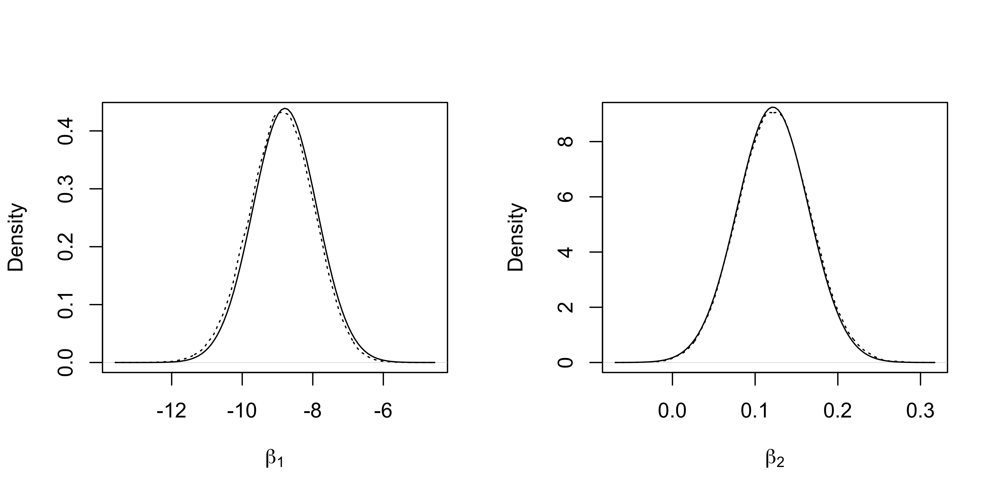

Further comparisons

We report the posterior means and variances under all the previous approximations and the gold standard MCMC values in the following.

Mean and variances

mu_MCMC <- colMeans(fit_MCMC)
Sigma_MCMC <- var(fit_MCMC)

Means <- data.frame(
  MCMC = mu_MCMC,
  Laplace = fit_Laplace$mu,
  VB = fit_CAVI$mu,
  HL = fit_HL$mu
)
knitr::kable(Means, digits = 4)

MCMC	Laplace	VB	HL
-8.8827	-8.7249	-8.7894	-8.7894
0.1229	0.1207	0.1215	0.1215
0.0345	0.0338	0.0341	0.0341
-0.0114	-0.0110	-0.0111	-0.0111
0.0080	0.0076	0.0078	0.0078
0.0753	0.0741	0.0745	0.0745
1.2425	1.2159	1.2282	1.2282
0.0249	0.0245	0.0247	0.0247

Sd <- data.frame(
  MCMC = sqrt(diag(var(fit_MCMC))),
  Laplace = sqrt(diag(fit_Laplace$Sigma)),
  VB = sqrt(diag(fit_CAVI$Sigma)),
  HL = sqrt(diag(fit_HL$Sigma))
)
knitr::kable(Sd, digits = 4, row.names = F)

MCMC	Laplace	VB	HL
0.9151	0.9049	0.6979	0.9086
0.0435	0.0430	0.0374	0.0431
0.0042	0.0041	0.0034	0.0041
0.0102	0.0101	0.0087	0.0101
0.0145	0.0145	0.0122	0.0145
0.0229	0.0225	0.0191	0.0226
0.3556	0.3522	0.2904	0.3533
0.0140	0.0138	0.0122	0.0138

Discrepancy from the optimal Gaussian

In the last table, we compute the Kullback-Leibler divergence between the obtained Gaussian approximations and the “optimal” Gaussian distribution, which matches the correct posterior mean and variance. These quantities are approximated using MCMC.

KL_gauss <- function(mu1, Sigma1, mu2, Sigma2) {
  p <- ncol(Sigma1)
  c(0.5 * (ldet(Sigma2) - ldet(Sigma1) - p + sum(diag(solve(Sigma2) %*% Sigma1)) + t(mu2 - mu1) %*% solve(Sigma2) %*% (mu2 - mu1)))
}

library(expm)
dWass_gauss <- function(mu1, Sigma1, mu2, Sigma2) {
  Sigma2_r <- sqrtm(Sigma2)
  c(crossprod(mu2 - mu1) + sum(diag(Sigma1 + Sigma2 - 2 * sqrtm(Sigma2_r %*% Sigma1 %*% Sigma2_r))))
}

tab <- data.frame(
  Type = c("Laplace", "Variational Bayes", "Hybrid Laplace"),
  KL = c(
    KL_gauss(fit_Laplace$mu, fit_Laplace$Sigma, mu_MCMC, Sigma_MCMC),
    KL_gauss(fit_CAVI$mu, fit_CAVI$Sigma, mu_MCMC, Sigma_MCMC),
    KL_gauss(fit_HL$mu, fit_HL$Sigma, mu_MCMC, Sigma_MCMC)
  ),
  Wasserstein = c(
    dWass_gauss(mu_MCMC, Sigma_MCMC, fit_Laplace$mu, fit_Laplace$Sigma),
    dWass_gauss(mu_MCMC, Sigma_MCMC, fit_CAVI$mu, fit_CAVI$Sigma),
    dWass_gauss(mu_MCMC, Sigma_MCMC, fit_HL$mu, fit_HL$Sigma)
  )
)
knitr::kable(tab, digits = 4)

Type	KL	Wasserstein
Laplace	0.0288	0.0257
Variational Bayes	0.2724	0.0613
Hybrid Laplace	0.0108	0.0090