Exercises A
Statistics III - CdL SSE
Author
Affiliation
Tommaso Rigon
Università degli Studi di Milano-Bicocca
Homepage
The theoretical exercises described below are quite difficult. At the exam, you can expect a simplified version of them; otherwise, they would represent a formidable challenge for most of you.
On the other hand, the data analyses are more or less aligned with what you may encounter in the final examination.
Data analysis
The dataset Abrasion, available in the MLGdata R package, comes from an experiment designed to evaluate how the abrasion resistance of a certain type of rubber is affected by its hardness and tensile strength. The original data are described in
Davies, O.L. and Goldsmith, P.L. (eds.) (1972) Statistical Methods in Research and Production, 4th Edition, Edinburgh: Oliverand Boyd, 239.
Thirty rubber samples were subjected to constant abrasion for a fixed duration, and the resulting weight loss (perdita, in grams per hour) was recorded. For each sample, the following variables were also measured:
D: hardness (in Shore degrees; the larger the number, the harder the rubber),
Re: tensile strength (kg/cm²).
Identify the statistical units, the response variable, and the explanatory variables, specifying the type of each variable (continuous quantitative, discrete quantitative, nominal qualitative, ordinal qualitative).
Perform a graphical analysis to assess whether a linear regression model may be appropriate.
Write the main equation of a simple linear regression model, choosing the most correlated explanatory variable.
Fit the simple linear regression model specified in point (c) in R.
Report the estimates and 95% confidence intervals for the coefficients. Interpret the estimated values.
For each element of the R
summaryoutput of thelmobject, indicate what quantity is being calculated and match it to the formulas in the slides/textbooks.Evaluate the goodness of fit of the model from (c). In particular, check if the variable omitted in the model specification is correlated with the residuals of the estimated model; comment the results. See also Exercise D (below) for a refined and alternative diagnostic plot.
Fit a multiple regression model in R including both explanatory variables. Interpret the estimated coefficients.
Evaluate the goodness of fit of the multiple regression model, using all the diagnostic tools at your disposal.
Obtain a 95% confidence interval for the mean weight loss when hardness is 70 Shore degrees and tensile strength is 180 kg/cm². For the same values, compute a 95% prediction interval for the response.
Littell et al. (2000) reported a pharmaceutical clinical trial involving n = 72 patients, randomly assigned to three treatment groups (drug A, drug B, and placebo), with 24 patients per group. The outcome of interest was respiratory function, measured as FEV1 (forced expiratory volume in one second, in liters). The source of the data is
Littell R. C., Pendergast J., Natarajan R. (2000). Modelling covariance structure in the analysis of repeated measures data. Statistics in Medicine, 19 (13), 1793-1819.
The dataset FEV.dat is available here. In this analysis, let y denote the FEV1 value after one hour of treatment (variable fev1 in the dataset). Define
- x_1: baseline FEV1 measurement prior to treatment (
base),
- x_2: treatment group (categorical variable
drugwith labelsa,b,p).
Import the data and then:
Fit linear models for y using the following sets of predictors: (i) x_1 only, (ii) x_2 only, (iii) both x_1 and x_2
Test to see whether the interaction terms are needed.
Check the underlying assumptions of the fitted models. If they are violated, propose a solution.
For each model, interpret the estimated parameters.
For n = 72 young girls diagnosed with anorexia, the dataset Anorexia.dat available here records their body weights (in lbs) before and after an experimental treatment period. The original source of the dataset is the textbook:
Agresti, A. (2015). Foundations of Linear and Generalized Linear Models. Wiley.
During the study, the participants were randomly assigned to one of three therapy groups:
- Control group: received the standard therapy (label
c),
- Family therapy (label
f),
- Cognitive behavioral therapy (label
b).
Import the data and
Fit a linear model where the outcome is the difference between the post-treatment weight and the baseline weight, and the predictor is the therapy group.
Check whether the assumptions underlying the fitted model are satisfied. If any assumption is violated, propose an appropriate remedy.
Interpret the estimated parameters of the model.
Test whether family therapy is effective in increasing weight.
Convert all weight measurements to kilograms (using the conversion factor 1\,\text{lb} = 0.453592 \text{kg}), repeat the analysis, and discuss whether and why the results change.
Theoretical
Prove that the variance-stabilizing transform for gamma random variables Y_i\sim \text{Gamma}(\alpha, \beta_i) with mean \mu_i = \alpha/\beta_i and variance \alpha/\beta_i^2, is the logarithm g(Y_i) = \log(Y_i).
Hint: use the fact that if Y_i \sim \text{Gamma}(\alpha, \beta_i) with mean \mu_i = \alpha/\beta_i and variance \alpha/\beta_i^2, then for large values of \alpha we have the approximation Y_i \; \dot{\sim}\;\text{N}(\alpha/\beta_i, \alpha/\beta_i^2).
In the linear model \mathbb{E}(Y_i) = \beta_1 + \beta_2 x_i, suppose that instead of observing x_i we observe x_i^* = x_i + u_i, where u_i is independent of x_i for all i, with \mathbb{E}(u_i) = \mu_u and \text{var}(u_i) = \sigma^2_u.
Analyze the expected impact of this measurement error on \hat{\beta}_1 and the residuals \bm{r}. What does it happen in the special case \mu_u = 0?
In some applications, such as regressing annual income on the number of years of education, the variance of Y_i tends to be larger at higher values of x_i > 0. Consider the model \mathbb{E}(Y_i) = \beta_1 x_i, assuming \text{var}(Y_i) = \sigma^2 x_i for unknown \sigma^2.
Show that the weighted least squares estimator minimizes \sum_{i=1}^n(y_i - \beta x_i)^2/x_i (i.e., giving more weight to observation with smaller x_i) and has \hat{\beta}_\text{wls} = \bar{y}/\bar{x}, with \text{var}(\hat{\beta}_\text{wls}) = \sigma^2 / \sum_{i=1}^n x_i.
Show that the ordinary least squares estimator is \hat{\beta} = (\sum_{i=1}^n x_i y_i) / \sum_{i=1}^n x_i^2 and has \text{var}(\hat{\beta}) = \sigma^2 (\sum_{i=1}^n x_i^3) /(\sum_{i=1}^n x_i^2)^2.
Show that \text{var}(\hat{\beta}) \ge \text{var}(\hat{\beta}_\text{wls}).
Hint: part (c) is not easy, but it can be solved in two ways: (i) by applying the Cauchy–Schwarz inequality to a suitable transformation of the x_i, or (ii) by relying on the Gauss–Markov theorem.
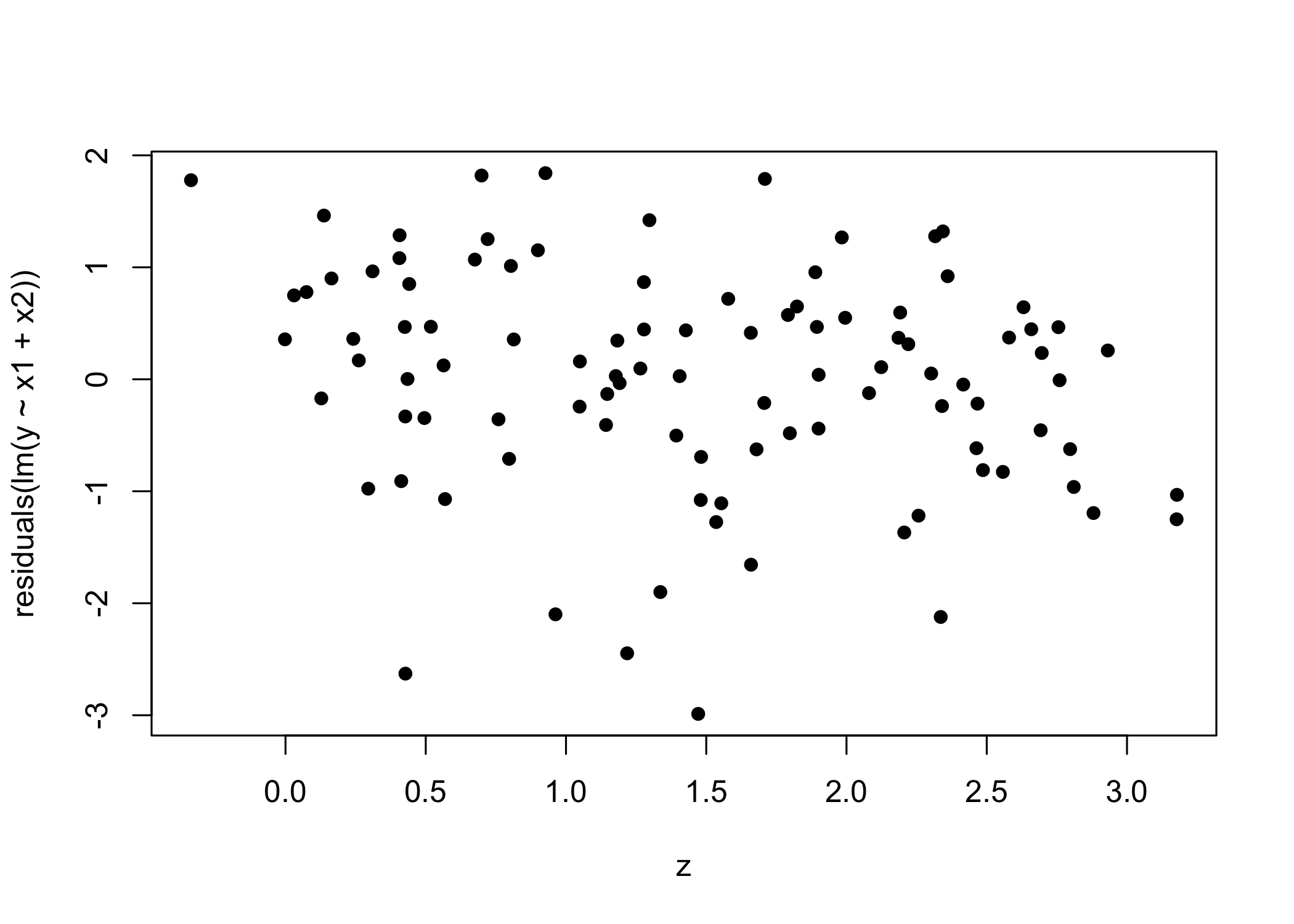
Suppose the normal linear model \bm{Y} = \bm{X}\beta + z\gamma + \bm{\epsilon}, with \bm{X} an n \times p matrix (rank p<n), \bm{z} an n \times 1 vector, and \bm{\epsilon} \sim \text{N}_n(0,\sigma^2 I_n). We instead fit \bm{Y} = \bm{X}\beta + \bm{\varepsilon}, with \hat{\beta} = (\bm{X}^T \bm{X})^{-1}\bm{X}^T \bm{y}, \qquad \bm{r} = (I_n - \bm{H})\bm{y}.
Show that \bm{r} = (I_n - \bm{H})\bm{z}\gamma + (I_n - \bm{H})\bm{\epsilon} so \mathbb{E}(\bm{r}) = (I_n - \bm{H})\bm{z}\gamma. What if \bm{z} lies in the column space of \bm{X}? What if \bm{z} is orthogonal to the column space of \bm{X}?
Explain why the added-variable plot (residuals from regressing \bm{z} on \bm{X} vs. residuals \bm{r}) helps assess whether to include \bm{z}.
Using the plots in the figure below, referring to the same set of data, comment on the results and suggest how to modify the model.
References
Agresti, A. (2015), Foundations of Linear and Generalized Linear Models, Wiley.
Salvan, A., Sartori, N., and Pace, L. (2020), Modelli lineari generalizzati, Springer.