  [1] 15  5 11 14  1  8 13  6 17  2 13 15  7 12  7  8  9  5  3  8  8  6  2 20 15
 [26] 20 13  8 15 11 12  4  3 15  3 11 14 20 14 14 11  7 11  1 11 14 17  1  2  7
 [51] 11 13  1  1 17 18  4  2  2  9 13 11 11  6  2  8 17  2 11  4 11  6  1 15 11
[76] 5 8 17 3 14 3 18 14 8 18 17 7 10 1 10 18 19 14 20 10 19 8 12 3 20Karmic dice for Baldur’s Gate III
A simple algorithm that accounts for karma
Karmic dice: what do they do?
I played the game “Baldur’s Gate” when I was a kid, on my old-fashioned computer and I thought it was a great game. When Baldur’s Gate III was released a few weeks ago, it caught my attention.
The central dynamic of the game is based on Dungeons & Dragons, meaning that players need to roll the famous 20 sided dice several times. On a laptop/console, these “random” numbers (actually, pseudo-random) are automatically generated by the software.
A specific feature of the game, the karmic dice, was very much discussed by the online community.
The karmic dice avoid subsequent successes and failures. In other terms, the results of the dice are not independent anymore.
I am an Assistant Professor of Statistical Science, so I had a few questions: how does this algorithm work, exactly? Will it preserve basic properties that do not screw up the balance of the game?
Perhaps more importantly: is it possible to find a simple way to generate “karmic” rolls?
Regular dice vs karmic dice
Let us step back for a second. Why do we need a karmic dice in the first place?
Most people find “true randomness” (independent trials, in the language of probability) quite counter-intuitive.
Suppose we toss a fair dice with 20 sides, say, 100 times. A compatible sequence of results could be:
A surprising amount of people would find this sequence “non-random” or would suspect that something is off with the random number generator (RNG). There is indeed a sequence of bad rolls: 7, 8, 9, 5, 3, 8, 8, 6, and 2. Is this some mistake?
Long story short: nothing fishy is going on, this is the normal behavior of a regular dice. Yet, a non-trained eye would expect something like the following karmic sequence (dependent trials):
  [1] 16 12  6 11  1  4 19  9  5 16  7 12 18  4 10 19  5 16  6 15  7  8 16 14 12
 [26] 13  8  2 20 15  7 20  5  8 14  2  9  5 15  7 20 14 12 13 14 16  1 17 20 12
 [51] 19 17 15  8 15  2 12 10  7 12 10  3  7  2 19 10  7  8 17 15 15 14  9 15 10
 [76] 15 10  3 10  4 14 19 19 16  7 15  4  5 13  5 11 12 19  8 14  9 20  8  9  3
In this sequence, there are fewer streaks of negative results, and many players find this kind of pattern more enjoyable.
The long-run behavior and weighted dice
There are many ways to obtain a sequence with fewer unlucky rolls. A simple idea could be using a weighted dice, e.g. an hypothetical dice with non-uniform probabilities.
Such a weighted dice accomplishes the goal of reducing extreme events, but it is modifying a fundamental aspect of Dungeons & Dragons and therefore affecting the balance of the game.
Changing the rules is not necessarily bad, but it has consequences. Indeed, most role players are well aware that there is a difference between 1d20 and 2d10.
Desiderata for a karmic dice
I think a more gentle approach would be tweaking the algorithm in such a way:
The long-rung proportions are identical to those of a regular dice, i.e., each side of the dice has a 5\% probability of being picked if we were to roll the dice a considerable amount of times.
The rolls are dependent, meaning the values obtained at the previous step influence future behavior.
Moreover, the algorithm should be easy to implement and tunable to account for players’ preferences (e.g., weak vs strong karma effect).
A simple algorithm for the karmic dice
I do not know which approach is implemented in Baldur’s Gate III, I can only make educated guesses. However, it turns out that a simple idea, based on the notion of latent karma, has all the above desiderata.
Let us focus on the generic tth roll. The latent karma Y_t of the is a real number that identifies how lucky we have been, say the positive values 1.5 or 3.2 (lucky events) or the negative value -4.3 (unlucky event).
Let 0 < \kappa < 1 be a constant determining the “karma effect.” The first karma score Y_1 does not depend on the past (because there is no past), and we generate it according to a Gaussian random variable:
Y_1 \sim \text{N}\left(0, \frac{1}{1 - \kappa^2}\right).
The subsequent karma scores are obtained by adjusting the previous karma score as follows:
Y_t = - \kappa \:Y_{t-1} + \epsilon_t, \qquad \epsilon_t \sim \text{N}(0, 1), for t = 2,\dots,n. In other words, if we were unlucky at step t, we had better chances to be lucky at step t+1 (and vice-versa). The amount of this effect is regulated by the parameter \kappa.
In R / python code, the generation of the latent karma scores is straightforward:
karmic_score <- function(n, kappa) {
  sigma <- sqrt(1 / (1 - kappa^2))
  latent_score <- numeric(n)

  # First latent karma Y_1
  latent_score[1] <- rnorm(1, 0, sigma)

  # Generation of the latent karma values Y_2,...,Y_n
  for (t in 1:(n - 1)) {
    latent_score[t + 1] <- -kappa * latent_score[t] + rnorm(1, 0, 1)
  }

  return(latent_score)
}
import numpy as np
def karmic_score(n, kappa):
sigma = np.sqrt(1 / (1 - kappa**2))
latent_score = np.zeros(n)
# First latent karma Y_1
latent_score[0] = np.random.normal(0, sigma)
# Generation of the latent karma values Y_2,...,Y_n
for t in range(1, n):
latent_score[t] = -kappa * latent_score[t - 1] + np.random.normal(0, 1)
return latent_scoreOnce we have obtained the karma scores Y_t, we simply convert them into integers D_t, belonging to 1,\dots,20, using the following formula
D_t = \text{ceiling}\{20 \Phi_\kappa(Y_t)\}, \qquad t = 1,\dots,n, where \Phi_\kappa(y) is the cumulative distribution function of a Gaussian with zero mean and variance 1 / (1 - \kappa^2).
The \text{ceiling} operation rounds up its argument, producing an integer. Once again, this operation can be performed with a few lines of R / Python code.
from scipy.stats import norm

def karmic_dice(n, kappa):
    sigma = np.sqrt(1 / (1 - kappa**2))

    # Generate the latent scores
    latent_score = karmic_score(n, kappa)
    # Convert the latent scores into integers between 1 and 20
    dice_results = np.ceil(20 * norm.cdf(latent_score, loc=0, scale=sigma))
    return dice_results
The usage of this function is also straightforward. In R, we can get a bunch of values for the latent score and the dice as follows:
Analyzing the algorithm
The most interesting property of this karmic dice is that it preserves the long-run proportions. If you have a solid background on the theory of auto-regressive processes and the so-called inversion theorem for generating random variables, this should be immediately obvious to you.
If you are not familiar with probability theory, the following empirical demonstration should give you an intuition of why this idea works nicely.
Suppose I were to get one million rolls, then I could check how many times I got each of the values 1,2,\dots, 20. With a computer, this can be quickly done (using \kappa = 0.35), and these are the proportions we get:
       1        2        3        4        5        6        7        8
0.049854 0.049871 0.049799 0.049926 0.050014 0.050330 0.050038 0.050022
       9       10       11       12       13       14       15       16
0.049772 0.049845 0.050407 0.050344 0.049760 0.050350 0.049981 0.049673
      17       18       19       20
0.050130 0.049961 0.049937 0.049986
Each number is roughly appearing in the sequence 5\% of the times, as it should!
The take-home message is that this algorithm does not affect the overall balance of the game because the long-term behavior (called stationary distribution) coincides with that of the regular dice.
The karmic effect
Another aspect we would like to understand is the dependence between the current roll and the following. These two rolls are independent in the case of a regular dice, but the situation is quite different in a karmic dice.
Let us start noticing that when \kappa = 0, the above karmic dice algorithm is just a convoluted way of sampling from a regular dice! It can be “easily” proved using standard probability tools.
When \kappa > 0, the karmic dice tweaks the probability and induces a negative correlation between subsequent rolls. Let us visualize what happens when \kappa = 0.35.
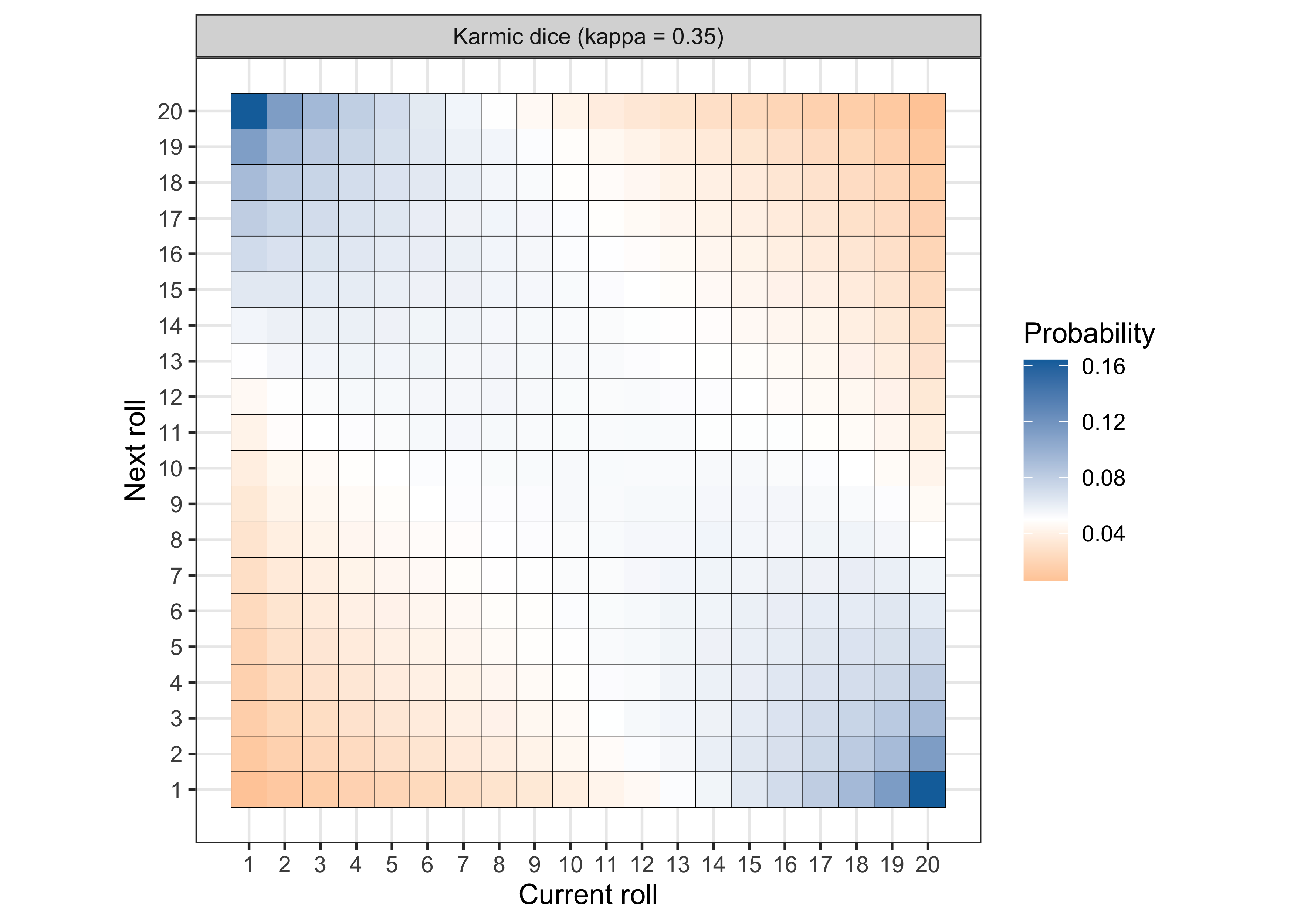
Blue squares are more likely values (compared to the regular dice), whereas orange squares are less likely values. This graph reveals a few interesting facts:
- If the current roll is a 1, then the most likely outcome of the following will be in the range of 15-20, with a peak in 20.
- If the current roll is 20, then the most likely outcome of the following will be in the range of 1-5, with a peak in 1.
- If the current roll is either 10 or 11, the following roll will roughly behave like a regular dice.
This version of the karmic effect therefore compensate positive values with negative values in a balanced manner so that the long-run proportions are correct.
The choice of \kappa
The amount of compensation is regulated by \kappa, a crucial tuning parameter that can be used to tune the dynamic of the karma dice.
If \kappa is close to 0, we get a regular dice. Vice versa, if \kappa is close to 1, i.e., the theoretical maximum, we would get sequences like this:
  [1]  7 13  7 14  7 14  7 14  7 13  8 13  8 13  7 13  8 13  8 13  8 13  7 14  7
 [26] 14  7 14  7 14  7 14  8 13  7 14  7 14  8 14  8 13  8 13  8 13  8 13  9 13
 [51]  8 13  8 13  8 12  8 12  9 12 10 11 10 11 10 11 10 11 10 11  9 12  9 12  9
 [76] 12  9 12 10 11 10 12 10 11 10 11 10 10 10 11 10 11 10 11 10 11 11 10 12 10
Even though, in the (very) long run, the correct proportions are still preserved for any \kappa < 1, such an extreme choice of \kappa = 0.999 leads to almost deterministic compensations, which are not appropriate for a game, because it would become too predictable.
There is no “statistical” optimal choice for \kappa, which instead should be selected based on the player preferences. Here I picked \kappa = 0.35 as it seems like a reasonable default, being a middle-ground solution between the independence case (regular dice) and an almost determinist pattern.